In the last step, a "Hamiltonian cycle" is a cycle in an undirected graph which visits each vertex exactly once.
Tractability and Approximation
In terms of growth order, polynomial-time algorithms are usually considered as tractable (efficient, affordable).
Complexity of algorithm vs. complexity of problem.
General representation: An abstract problem Q is a binary relation on a set I of problem instances and a set S of problem solutions. It becomes a concrete problem when every instance is represented by a binary encoding, with the length of the string taken as the size of instance.
A decision problem: a solution is "yes" or "no". Many other types of problems can be casted into a related decision problem that is no harder. For example, an optimization problem "Find the shortest path" can be casted into decision problem "Does the shortest path have length k?".
A decision problem is often represented by a formal language whose sentences corresponds to problem instances whose answer is "yes". In this way, "to solve a decision problem" becomes "to decide whether a language accepts a sentence". A complexity class is a class of languages of a certain complexity.
The complexity class P is the class of languages that can be decided by a polynomial-time algorithm, i.e., there is a constant k such that for any length-n binary string x, algorithm A correctly accepts or rejects x in time O(nk).
The complexity class NP is the class of languages that can be verified by a polynomial-time algorithm. A two-argument algorithm A verifies an input string x if there exists a certificate y (which is also a binary string) such as A(x, y) = 1. Intuitively, the algorithm A uses the certificate y to prove that x is in L.
Obviously, P ⊆ NP, but whether P = NP is a pending problem.
A problem P can be reduced to another problem Q if any instance of P can be mapped into an instance of Q, and the solution to Q provides a solution to the instance of P. A language L1 can be reduced into a language L2 in polynomial time, we have L1 ≤p L2. In this situation, if L2 is in P, so is L1.
A binary language L is "NP-complete" (or "in NPC") if it is in NP, and every NP problem can be reduced to it. Defined in this way, if any language in NPC is also in P, then P = NP.
Since there are already many known NPC problems, we can prove a new NP problem belongs to this category by reducing (in polynomial time) a known NPC problem into it.
So far, all known algorithms of NPC problems take exponential time, so these problems are considered as "intractable" or "hard". Most people believe that P and NPC are two subsets of NP that have no common element. However, it hasn't been proved yet.
Example of NPC problems: Traveling-Salesman Problem (TSP). Given a weighted undirected graph, G, a tour is a path that goes through each vertex exactly once and finally return to the starting point. The original TSP is to find the shortest tour in a complete graph (where there is an edge between every pair of vertices), while the related decision problem is to find a tour within a given total weight k. This problem is in NP because given a graph and a tour, it is easy to check whether the tour satisfies the requirement; it is in NPC because a known NPC problem, Hamiltonian Cycle, can be reduced into it. This problem can be solved by exhaustively generating all possible tours, but that will use exponential time.
For an optimization problem, an approximation ratio ρ(n) is often used to indicate the closeness of an approximate solution to an optimal solution. For any input of the size n, if actual solution is C and the optimal solution is C*, and max(C/C*, C*/C) ≤ ρ(n), the algorithm is called a ρ(n)-approximation algorithm.
Usually there is a trade-off between computation time and the quality of the approximation.
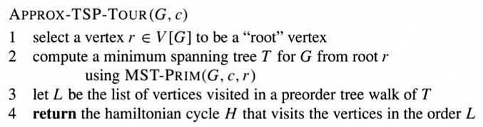
For example, if in a Traveling-Salesman Problem (TSP) we can assume the triangle inequality, that is, a direct path is never longer than an indirect path, then an approximate solution can be obtained by first building a minimum spanning tree for the graph, then planning a tour based on the tree.
In the last step, a "Hamiltonian cycle" is a cycle in an undirected graph which visits each vertex exactly once.
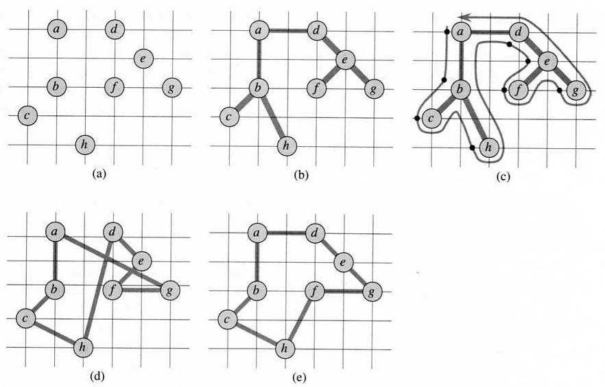
In the following example, the actual distance between vertices is used as the weight of the edge connecting them. The first four figures show how the algorithm works step by step, while the last one shows an optimal solution.
The running time of Approx-TSP-Tour is polynomial.
To evaluate the approximation ratio of Approx-TSP-Tour, we consider the following items: