Probabilistic Analysis and Randomized Algorithms
The actual probability distribution is usually domain-specific, and not a property of the algorithm.
When all instances have the same probability (i.e., 1/m), the average cost is ∑[i = 1..m] (1/m)ci = (∑[i = 1..m] ci) / m.
For linear search, if the target value has the same probability to appear in any positions in an array, then what is the average number of comparisons? Consider the following three cases:
Cost as exact function, approximate function, and order of growth: when to use which?
How about binary search?

The quantity to be analyzed is the cost of the procedure, reflected by line 3 and 6, not the running time of the algorithm. However, the analysis is similar: we want to know the number of times for line 3 and 6 to be executed, respectively.
Assuming the cost of interviewing and hiring are ci and ch, respectively, the cost of the above algorithm is n ci + m ch, where m is the number of hiring. Since the interview cost n ci remains unchanged, our analysis will focus on the hiring cost m ch, therefore, m.
What are the best case and the worst case?
Candidate i is hired exactly when he/she is the best in 1 through i. If the candidates come in random order, then the probability for that event is 1/i. Therefore the expected number of hires is the sum of a harmonic series ∑[i = 1..n] 1/i = ln n + O(1) (A.7, page 1060, 1066). As a result, the average hiring cost of the algorithm is O(lg n).
What if hiring can only happen once? The hiring cost will be minimized, though it can no longer guarantee to hire the candidate with the highest quality.
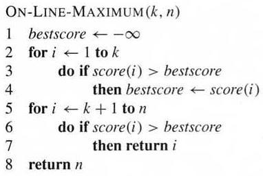
One solution: first select a positive integer k < n, interview but reject the first k candidates, then hire the first candidate thereafter who has a higher score than all the preceding candidates. If no such one can be found, hire the last one.

What is the best choice of k that gives the highest probability for the best candidate to be hired?
Call that probability Pr{S} and divide it into the events where the hiring happens when the best candidate is at position i: Pr{S} = ∑[i = 1..n] Pr{Si}. Since the first k candidates are all rejected, it is actually ∑[i = k+1..n] Pr{Si}.
The event Si happens if and only if (1) the best candidate is at position i, and (2) nobody before it is better than the best of the first k candidates. The first value is 1/n, and the second one is k/(i-1). In summary,
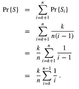
Pr{S} is maximized when k = n/e, with the value 1/e (page 116-117).
Many randomized algorithm randomize the input by permuting the given input array A. One common method for doing so is to assign each element in the array A[i] a random priority P[i], and then sort the elements of A according to their priorities:
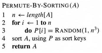
The range [1, n3] makes it likely that all the random numbers produced are unique.
Another method for generating a random permutation is to permute the given array in place. In iteration i, the element A[i] is chosen randomly from subarray A[i..n], then remain unchanged.

It can be proven that both algorithms generate random permutation as desired. Which is more efficient?
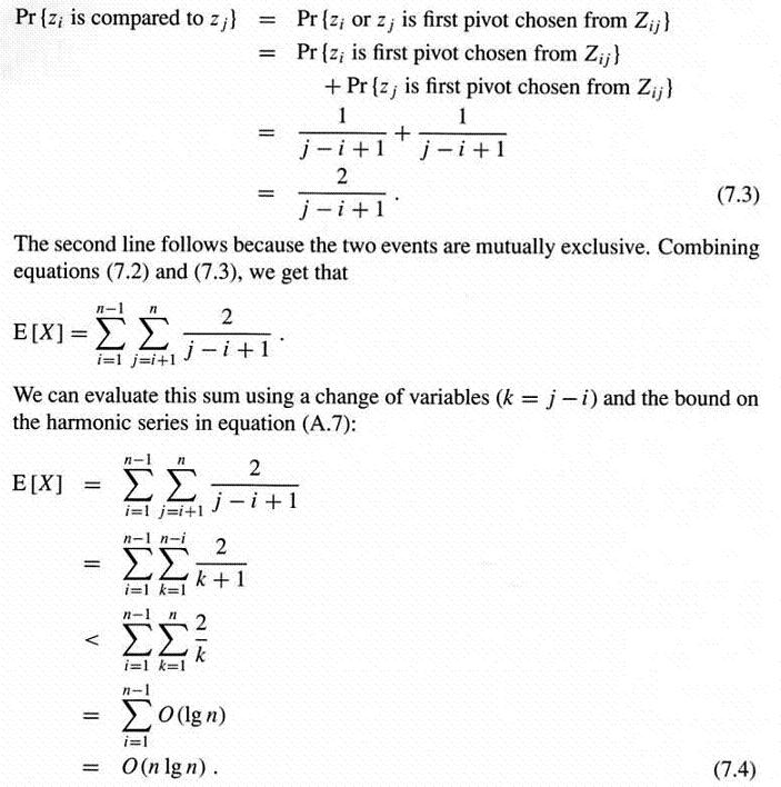
The cost comes from the number of comparisons, which is the sum of probability of every pairwise comparisons. Let zi and zj be the ith and jth smallest values, and Zij be the set containing them and the values in between, then
