1. Solving problem with algorithm

Algorithm: a (finite and predetermined) sequence of (directly executable or already defined) computational steps that produces an output for a valid input in finite time.

Desired properties of algorithm, as a solution to a problem:

• correctness: satisfying problem specification
• efficiency: low time and space expense
• simplicity: conceptual naturalness and length of description

Programming: to implement an algorithm in a computer language.

2. Time efficiency analysis

• the problem-solving method of the algorithm,
• the concrete problem instance it is given,
• the software and hardware in which the algorithm is implemented and executed.

1. assuming constant time cost for each type of computational step, then only count the number of steps,
2. measuring the size of instance, usually by length of description,
3. for a given size, only considering the worst case (or average case, best case) situation,
4. measuring the efficiency (time complexity) of an algorithm in a situation as a function of instance size,
5. only considering how fast the function value increases as size increases,
6. classifying functions into categories by order of growth.

The asymptotic efficiency of algorithms, represented by a simple function g(n):

• Θ(g(n)) = {f(n) : there exist positive constants c₁, c₂, and n₀ such that 0 ≤ c₁g(n) ≤ f(n) ≤ c₂g(n) for all n ≥ n₀} — g(n) is an asymptotic bound of f(n).
• O(g(n)) = {f(n) : there exist positive constants c and n₀ such that 0 ≤ f(n) ≤ cg(n) for all n ≥ n₀} — g(n) is an asymptotic upper bound of f(n).
• Ω(g(n)) = {f(n) : there exist positive constants c and n₀ such that 0 ≤ cg(n) ≤ f(n) for all n ≥ n₀} — g(n) is an asymptotic lower bound of f(n).
• o(g(n)) = {f(n) : for any positive constant c > 0, there exist a constant n₀ > 0 such that 0 ≤ f(n) ≤ cg(n) for all n ≥ n₀} — g(n) is a upper bound of f(n).
• ω(g(n)) = {f(n) : for any positive constant c > 0, there exist a constant n₀ > 0 such that 0 ≤ cg(n) ≤ f(n) for all n ≥ n₀} — g(n) is a lower bound of f(n).

To decide the relation between two functions:

• f(n) = o(g(n)) if and only if Lim[f(n)/g(n)] = 0.
• f(n) = Θ(g(n)) if and only if Lim[f(n)/g(n)] = c (a positive constant).
• f(n) = ω(g(n)) if and only if Lim[f(n)/g(n)] = ∞.

The major growth orders, from low to high, are:

• constant: Θ(1)
• logarithmic: Θ(log_an), a > 1
• polynomial: Θ(n^a), a > 0 — further divided into linear (Θ(n)), quadratic (Θ(n²)), cubic (Θ(n³)), and so on
• exponential: Θ(aⁿ), a > 1

3. Analysis of recurrences

Recursion: part of a problem is a simpler problem of the same type.

Assume the algorithm

1. directly solves problems instances in constant time if their size is smaller than a constant c,
2. otherwise uses D(n) time to divide a problem into number a of smaller subproblems of the same type, each with 1/b of the original size,
3. combines their solutions in C(n) time to get the solution for the original problem,

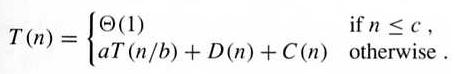
To solve a recurrence:

1. substitution method: use mathematical induction to prove a function that was guessed previously;
2. recursion tree method: represent the equation as a tree to reveal the function — the height of the tree is log_bn, and the number of leaves is a^log_bn (same as n^log_ba);
3. the master method:
   
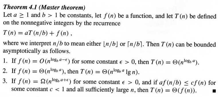
   In the recursion tree, the three cases correspond to different relative cost spent on root/leaves.

   As a special case, when a = b, log_ba = 1, and there are n leaves. The above results are simplified to (1) Θ(n), (2) Θ(nlgn), and (3) Θ(f(n)), respectively.