1. Average cost

As a special situation, when all instances have the same probability to show up, that is, p_i = p. Since ∑_{[i = 1..m]} p_i = 1, then ∑_{[i = 1..m]} p_i = mp = 1, so p = 1/m, and the average cost ∑_{[i = 1..m]} p_ic_i = (∑_{[i = 1..m]} c_i) / m.

To get the probability values is not always easy. Usually, they are based on the knowledge and assumptions about the problem instances to be processed, so are application-dependent and not a property of the algorithm itself, except under idealized assumptions.

2. Example: the hiring problem

This example has some unusual properties:

• As a practical problem, the steps are not fully formalized.
• The goal is to analyze the cost of the procedure, reflected by line 3 and 6, not the running time of the algorithm.
• The input does not have to be available at the same time (at the very beginning), and the output does not have to be available at the same time (at the very end), neither.

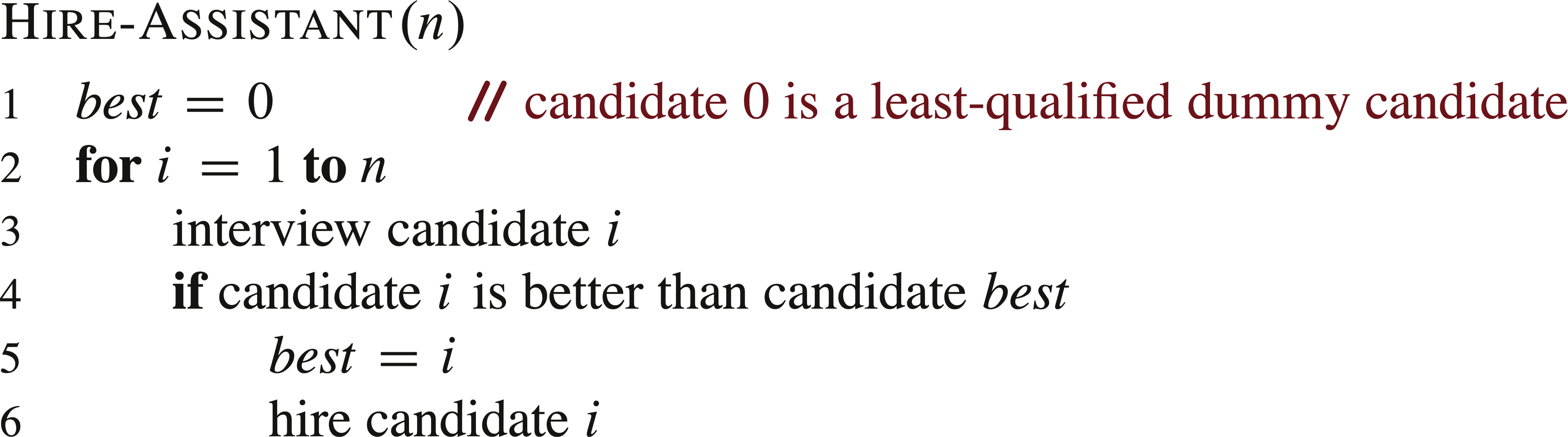
Obviously, for this problem the best case happens when the best candidate comes first (m = 1), and the worst case happens when every candidate is better than the previous ones (m = n).

To calculate the average hiring cost, we assume that the candidates come in random order, meaning that each possible order is equally likely. Please notice that such an assumption is different from a "complete ignorance" or "pure arbitrary" assumption --- which assumes that we don't know which input instance the algorithm will meet each time, but we do know that in the long run all possibilities will happen equally often. In general, it is not always valid to treat a variable with an unknown value as a random variable in this sense.

To calculate the probability for line 6 in the above algorithm to be executed, we can see that candidate i is hired exactly when he/she is better than all candidates 1 through i − 1. Assuming any one of the first i candidates is equally likely to be the best so far, candidate i has probability of 1/i to be hired. The expected number of hires is ∑_{[i = 1..n]} 1/i = ln n + O(1), which is O(ln n) (Page 1142, equation A.9).

3. Randomized algorithm

One way to avoid this situation is to actually impose a probabilistic distribution onto the input, so as to turn it into a random variable. The common way to do so is to use a pseudo-random-number generator to rearrange the input. In this way, no matter how the input is presented to the system, the average computational cost is guaranteed to fit the probabilistic analysis. Such an algorithm is called "randomized". Please note that this solution assumes that all candidates are all available for processing at the very beginning, as well as that the hiring process will be repeated for many times.

For such a randomized algorithm, no particular input always has the best-case, or the worst-case, of time cost.

Many randomized algorithms work by shuffling the given input array A. One way to do so is to assign each element in the array A[i] a random priority P[i], and then sort the elements of A according to their priorities:

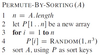
The range [1, n³] is chosen to reduce duplicates in the random numbers generated.

A better method for generating a random permutation is to permute the given array in place. In iteration i, the element to be put at A[i] is chosen randomly from subarray A[i..n], then remain unchanged.

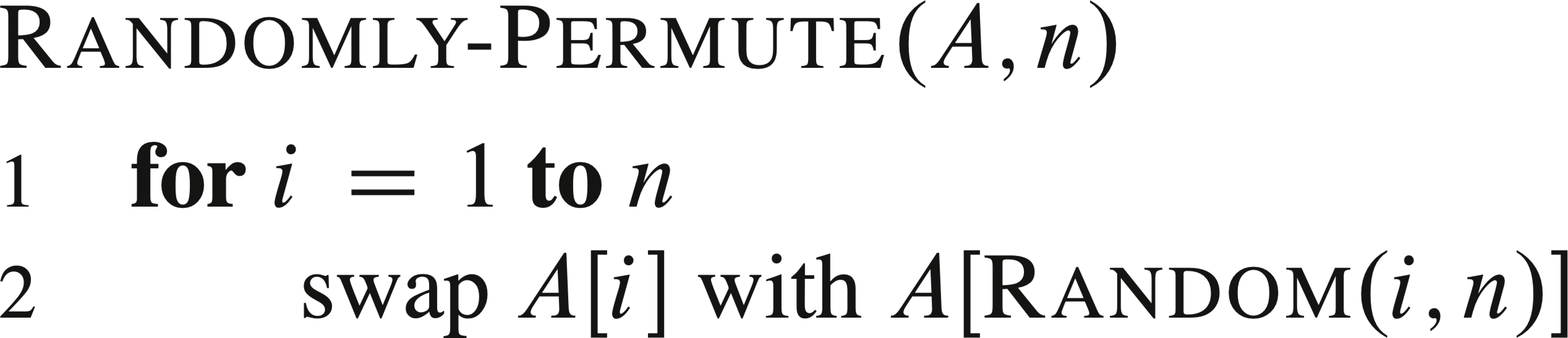
It can be proven that both algorithms generate random permutation as desired. For why the Random(i, n) cannot be replaced by Random(1, n), see this explanation.

4. Example: the on-line hiring problem

For this new problem, what is the trade-off between minimizing the amount of interviewing and maximizing the quality of the candidate hired?

Let's assume that after an interview we can assign the candidate a score, and no two candidates have the same score. One solution is: first select a positive integer k < n, interview but reject the first k candidates, then hire the first candidate thereafter who has a higher score than the best of the first k (which is also the best of all the preceding) candidates. If no such one can be found, hire the last one.

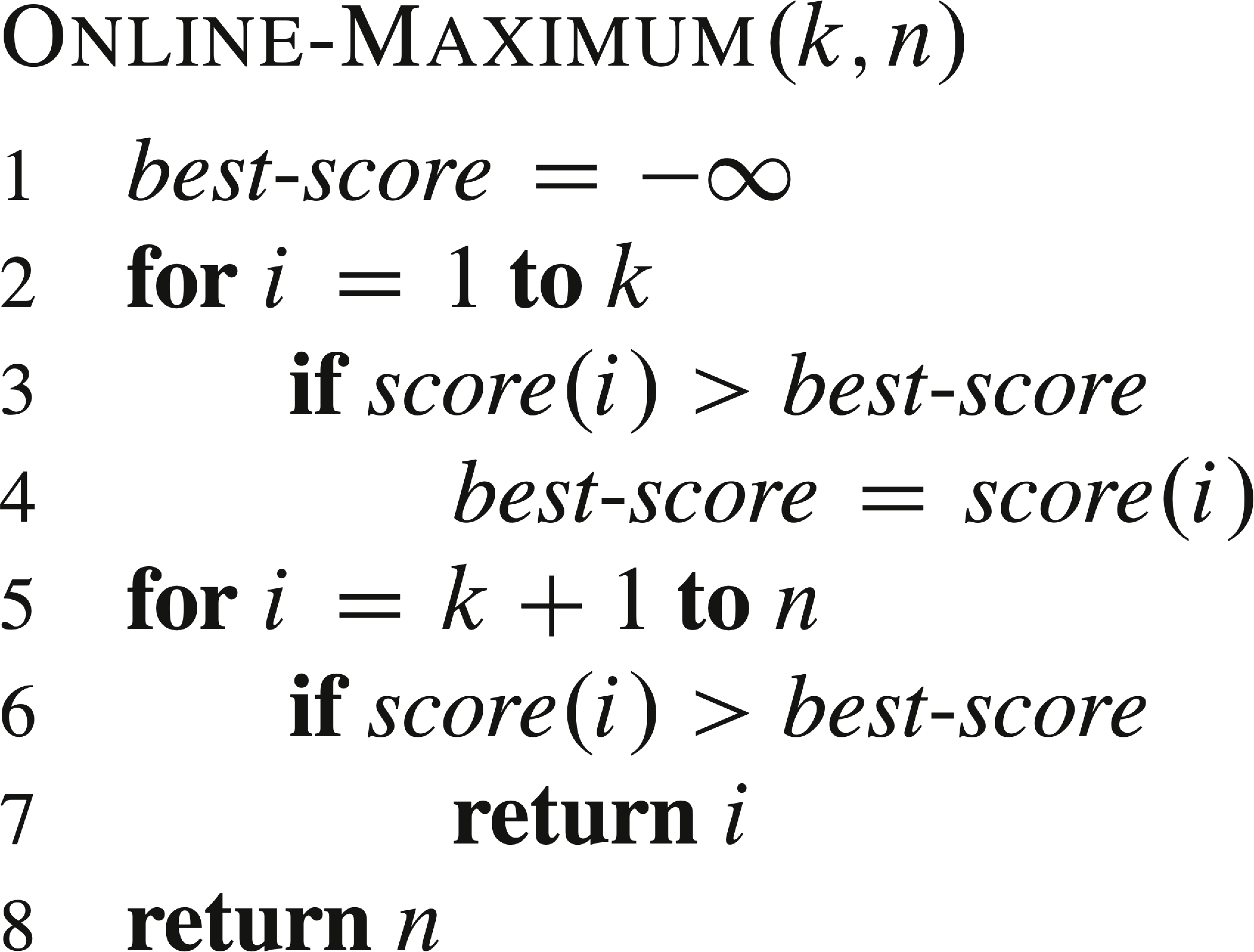
Now the problem is to decide the best choice of k. Here we define it as the value that gives the highest probability for the best candidate to be hired, Pr{S}. This event is the summation of the events where the hiring happens when the best candidate is at position i: Pr{S} = ∑_{[i = 1..n]} Pr{S_i}. Since the first k candidates are all rejected, it is actually ∑_{[i = k+1..n]} Pr{S_i}.

The event S_i happens if and only if (1) the best candidate is at position i, and (2) nobody before it is better than the best of the first k candidates. Under the assumption of equal probabilities, the first value is 1/n, and the second one is k/(i − 1). In summary,

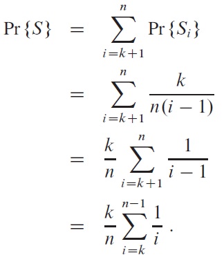
It can be proved (see textbook page 152) that Pr{S} is maximized when k = n/e, with the value 1/e (about 37% or 1/3).

Please note that the above Pr{S} is just one of the possible ways to define the optimal result.

Related topics:

• Feynman’s Restaurant Problem
• The multi-armed bandit problem
• Exploration vs. exploitation