John P. Dougherty
jd@zoro.cis.temple.edu
voice: 215.842.9535 fax: 215.483.3146
Yuan Shi
Department of Computer and Information Science
shi@falcon.cis.temple.edu
voice: 215.204.6437 fax: 215.204.5082
Temple University
Philadelphia, Pennsylvania 19122
Application development for distributed and parallel processing is significantly more complex than its sequential counterpart. Coarse-To-Fine graphs, or CTF graphs, can be utilized to represent distributed applications and identify fundamental parallel structures. This performance based decomposition tool emphasizes simplicity, only adding detail when a performance contribution is realized. This report supports CTF as a philosophical approach for application design, as well as demonstrates the usefulness of CTF graphs for an extensive range of applications.
Keywords: decomposition techniques, rapid prototyping,
parallel programming
1.0 INTRODUCTION
Coarse-grained distributed computing has grown in popularity while other forms of parallel processing have encountered obstacles [Lewis 1994]. Using existing topologies of (nondedicated) workstations and networks, this form of parallel processing is manifested in cluster computing, symmetric multiprocessing, and even client-server computing [Pfister 1995]. Application development is significantly more complex than sequential programming [Carriero and Gelernter 1989], mandating tools to decrease development time (and costs). Currently there are no tools that can identify the proper "coarseness" of a parallel application using a deterministic approach.
Coarse-To-Fine (CTF) Graphs are high-level dependency graphs used to represent the essential features of a target distributed application. CTF graphs provide the starting point for such endeavors as distributed application design [Shi 1995] and performance/dependability analysis (a.k.a., steady-state performability analysis [Dougherty 1995b]); it is believed that these graphs will be used for parallel compilation in the future [Shi 1993].
This manuscript demonstrates the usefulness of CTF graphs for distributed application representation. After some preliminary definitions, a CTF graph will be developed for a sample application, Monte Carlo Integration, along with performance, execution time, availability, and performability metrics. Next, CTF graphs will be placed into context for distributed application design and analysis, as well as look at future objectives. As an appendix, a series of CTF graphs will be developed for a diverse set of distributed applications.
2.0 CTF GRAPH PRELIMINARIES
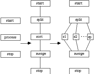
After formally defining a CTF graph, the discussion proceeds to construction and analysis. CTF graphs are based on vertex series-parallel (VSP) digraphs [Valdes et. al. 1982]. VSPs have been utilized for probabilistic performance and dependability analysis [Sahner and Trivedi 1987]. VSPs are constructed through the recursive application of two composition rules: a series composition rule and a parallel composition rule. For CTF graphs, the composition rules are detailed further into four.
The application developer should remember that CTF construction implies distributed application decomposition.
2.1 Definitions
A Coarse-To-Fine Graph, or CTF graph, is an acyclic directed graph
G = {V,E}
where
V = a finite set of processes
E = a dependency relationship, usually interprocess communication
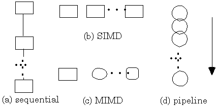
For most programs, loops are the construct which generate most of the need for compute cycles. SIMD and MIMD exploit patterns found in the control and/or data streams to process these loops.
In practice, CTF graphs are constructed quite differently than VSPs. CTF graphs are generated during the initial stages of the design of a distributed application using a "coarse-to-fine approach (CTF). CTF dictates that simplicity is favored over detail in hopes of obtaining reasonable accuracy rapidly.
The construction rules for CTF graphs are recursively defined as follows:
(i) a single vertex (i.e., process) is a CTF graph
(ii) given two existing CTF graphs G1 = <V1, E1> and G2 = <V2, E2>, then the graph G is also a CTF graph if constructed using
(a) sequential construction: Gseq = <V1UV2, E1UE2U(T1xS2)>, where T1 is the set of sinks of G1 and S2 is the set of sources of G2 for a fixed data stream.
(b) pipe construction: Gpipe = <V1UV2, E1UE2U(T1xS2)>, where T1 is the set of sinks of G1 and S2 is the set of sources of G2 for a continuous data stream.
(c) simd construction: Gsimd = <V1UV2, E1UE2>, and all the vertices execute the same control stream (i.e., execute the same process on different data)
(d) mimd construction: Gmimd = <V1UV2, E1UE2>, and the vertices can execute different control streams (i.e., execute different processes on different data)
2.2 Construction and Analysis Methodology
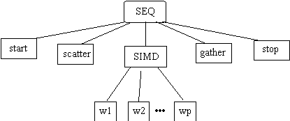
These elements for CTF graph composition are depicted in Figure 1.
There exist other distributed - parallel programming approaches which begin with a detailed (data and/or functional) decomposition of the target application and attempt to group pieces together for the target distributed environment. Examples include chunking [Pfister 1995, p. 222] and the agglomeration phase of the PCAM (Partition-Communication-Agglomeration-Mapping) approach [Foster 1995, p.42]. Contrary to these approaches, it is proposed here that the most appropriate technique for design is a coarse-to-fine decomposition. Development starts with the simple, adding detail only when this detail contributes to performance of the implemented program.
The initial phase of CTF graph construction is easy; each applications begins as a single vertex. The remaining phases of CTF graph construction involve i.) when to build (i.e., decompose); ii.) which construction element to use; and iii.) when to terminate this process. These three aspects will now be discussed at length.
2.2.1 Loops - Sources of Concurrency
It can be argued that computational work is found primarily in loops. Program code devoid of loops does not contain a significant amount of work to mandate any attention for CTF decomposition. The main reason is the significant advances in processor technology; even a sequential portion of code consisting of a million operations would need only (about) one second on a 1 MFLOPS machine.
Loops are candidates for the parallel CTF construction elements. The primary determining characteristic is dependency among iterations. Loops with dependent iterations can (possibly) utilize MIMD or pipe constructs to overlap processing in time and increase realized performance. This is sometimes referred to as functional decomposition [Foster 1995].
Loops containing independent iterations can be further divided into apriori (i.e., for loops) and aposteriori (i.e., while loops). Examples of applications that fall into the former category include Monte Carlo algorithms, image processing, and matrix applications. The distinguishing feature of the latter category is usually convergence; computation iterates until some condition becomes true. Many searching applications and scientific applications contain while loops.
Nested loops are encountered for many, if not most, computationally-dense applications. Computational complexity has demonstrated the impact of nested loops [Korsh 1986]. CTF decomposition of nested loops is a nontrivial issue discussed in the following section.
2.2.2 CTF Graph Element Selection
The previous section argued the rationale of decomposing applications at the loops. This section will detail the selection of the CTF graph construct for loop decomposition. It is important to remember that this methodology considers a target application for a given processing environment.
The discussion begins with independent iterations implemented using SAG. Consider an apriori loop which iterates N times on P processors, N >> P. For CTF graph construction (and parallel programming), independent iterations provide the greatest source of concurrency to exploit. SIMD is used to distributed the iterations among the P processes. Experience reported here and in [Horowitz and Zorat 1983; Shi 1991, Parhami 1995] has demonstrated that SIMD is the most frequently used element. Given independent iterations, a simple Scatter-And-Gather (SAG) approach is best. Each application in section A1 in the appendix utilizes SAG.
Nested independent loops are decomposed starting with the outermost loop. Given the following program segment,for i = 1 to N1 for j = 1 to N2 for k = 1 to N3 ï ï ï
CTF dictates partitioning the N1 iterations of the i loop.
While SIMD is utilized within a loop (or set of nested loops), MIMD and pipe are used to exploit concurrency among loops. If neither a control dependency or a data dependency exists among a set of loops, then it is prudent to introduce a MIMD construct. Experience in this report has found this case to be rare.
The final construct, pipe, is applied when there is a control dependency among a set of process but not necessarily a data dependency. The requirement for a pipe construct is a continuous stream of data input to the application. A pipe overlaps different control pieces (i.e., stages) so that overall performance is enhanced.
2.2.3 Termination Criterion
As with many recursive strategies, a termination criterion must be established. CTF favors simplicity over detail [Shi 1993; Dougherty 1995b]; more importantly, CTF graph construction stops when the available concurrency has been exhausted. Limits on the degree of parallelism are found in either the application or the environment (or both).
For example, given P processors, i.) an SIMD construct can have no more than P components; ii.) an MIMD construct can have no more than P pieces; and iii.) a pipe construct can have no more than P stages. This is an illustration of an environmental limit.
It will be shown later (section A.6.3) that a Navier-Stokes application can be represented as a CTF graph with an MIMD construct; this construct is limited by the fact that only two processes can be executed in parallel, no matter how many processors are available. This is an illustration of an application limit.
2.3 Performance Analysis
Once a distributed application has been decomposed into its constituent parts, and the dependency relationships among these parts has been detailed, a decomposition tree can be generated. In this tree, the vertices of the CTF graph become leaves, and internal nodes represent the construction element used. In this way, nested CTF structures can be studied.
2.3.1 Decomposition Trees
To demonstrate this transformation of a CTF graph into a decomposition tree, consider Figure 2 below.
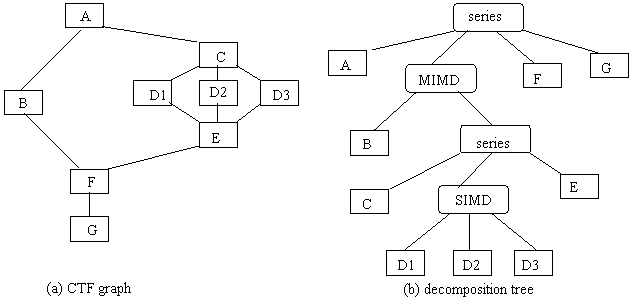
Techniques for developing decomposition trees are given in [Sahner and Trivedi 1987]. The vertices from the original CTF graph become leaves in the decomposition tree, while the internal nodes of the tree are specified by the construction element among the children processes.
2.3.2 Traversal and Analysis
Since the graph is acyclic, the tree is certain to
be finite. Using postorder traversal, performance, execution time,
availability and performability data can be obtained for each
component. The analysis rules for the traversal are given in Figure
3.
| Perform | ance | ||
| Internal Node | |||
| sequential |  } } | ||
| SIMD (no FT) |  | ||
| SIMD (FT) |  | ||
| MIMD |  | ||
| pipeline |  } } |
Timing Models [Shi 1994] can be utilized to obtain expected performance information. Execution time estimates are collected directly from algebraic equations which specify the application and environment parameters. In this way, the development time can be reduced by identifying bottlenecks early. Section 3.3 demonstrates how Timing Models can be used to predict a lower bound for a distributed application.
Steady-State Performability, or SSP, is an extension of Timing Models to include dependability issues into the definition of performance [Dougherty 1995b]. Performability analysis is somewhat more complex. Timing Models use time as the chosen metric; however, dependability and performability analysis using time can encounter a singularity for the application state when all processes are down (i.e., time = _). This is why Figure 3 includes both performance and time.
For SSP, availability indicates the percentage of time a process is delivering work to the application, and can be determined as
a = [1]
From the Binomial Theorem, the percentage of time that an application remains in state i, where i indicates the number of processes delivering service (i e [0, M]), is given by]
Ai = ai (1-a)(M-i) [2]
Once this notion of availability is defined, performability can be defined for a distributed application. In essence, performability analysis, as seen in Markov Chains, looks at the possible states that an application reaches, and the performance delivered at each state. Performability becomes a simple summation of the performance provided at each state multiplied by the percentage of time that the application spends in that state, or
PA(M) = [3]
From Figure 3, the only CTF element which needs this previous formula is SIMD using a fault tolerant protocol such that the work of a failed process is completed by one of the remaining processes. With the other constructs, the process only delivers performance if all processes are available, reducing [3] to
PA(M) = P(M) ï A(M) [4]
The success of both of these analysis methods hinges on a deterministic technique for decomposing a distributed application, and CTF graphs provide that technique.
2.4 Finitely-Cyclic Applications
There are certain applications (e.g., Asynchronous Linear System Solver, HiTech Chess) which follow a Computer-Aggregate-Broadcast paradigm [Nelson 1987]. In this case nested loops can exist, but they are dependent in that the results at the end of an iteration of the outermost is needed among the constituent components of the next iteration. CTF graphs can be designed using one of two possible methods.
In the first case, the amount of work is "reasonable" among these nested loops. Reasonable in this context implies that it is possible to represent the nested loops as a single vertex without losing any chance to exploit concurrency. Such reasonable amount of computational effort (nested or not) would not mandate a separate CTF graph construct.
However, the more interesting case is where there is a significant amount of computational work within the inner loop(s), or whatever set of constructs are present. In this case, a cycle must be introduced into the CTF graph. For implementation issues, this cycle does not generate additional difficulty; on the other hand, analysis techniques such as steady-state timing models [Shi 1995] and steady-state performability [Dougherty 1995a] mandate that the number of times this cycles is traversed be finite.
However, certain applications mandate that finite cycles be incorporated into CTF graphs, namely Compute-Aggregate-Broadcast (CAB) applications [Nelson 1987]. For analysis, the number of iterations must be finite and know (or estimated) beforehand. In most cases, the cycle count C is set to either the upper bound or the average number of cycles expected.
The remainder of this document surveys a number of distributed applications and shows the steps needed to develop a CTF graph for each. Dividing this application survey into distinct categories is difficult because each applications contains its own combination of features. However, in the name of "readability", applications are partitioned into the categories of i.) "embarrassingly-parallel", ii.) sorting, iii.) searching, iv.) numerical, and v.) coarsely-iterative.
3.0 MONTE CARLO INTEGRATION EXAMPLE
This numerical technique is utilized to integrate a function over a region which may not be easy to sample randomly, possibly due to the complexity of the shape of the region. Monte Carlo Integration (MCI) uses random numbers to approximate the value of an integral [Press et. al. 1987]. The greater the number of random points generated, the more accurate the approximation. Partitioning this work involves little communication overhead since only a signal (possibly a seed) needs to be sent to a process.
3.1 CTF Graph
Using SAG, the following CTF graph is generated:
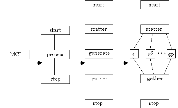
3.2 Decomposition Tree
Detail is added to the graph as needed; in this case, detail is required in the process block to uncover the parallelism among the worker processes, which impacts both performance and availability. Another attractive feature of this application is that it is complete devoid of cycles, making the corresponding decomposition tree directly evident. The tree is depicted in Figure 5 below.
3.3 Traversal and Analysis
Timing Models and SSP analysis of the decomposition tree from Figure 3 involves postorder traversal using a set of analysis rules [Dougherty 1995b]. Analysis will include performance (processing rate P and execution time T), availability A and performability PA.
Postorder traversal of Figure 5 results in the following parallel execution time and performance models,
Tpar = Tstart + Tscatter + Tprocess(SIMD) + Tgather + Tstop [5]
From this equation the expected execution time for the MCI application is determined by summing the component execution times. These times are readily available from Timing Models, which are discussed in the next section. When dependability issues are introduced into this situation, an tool such as SSP can be used; this is discussed in the section after Timing Models.
3.3.1 Timing Models
Assuming that the time for the processes Tstart, Tscatter, and Tstop are insignificant, they will all be set to zero. This is reasonable since each involves a brief sequential process to be executed by the master component of the SAG organization used for MCI. For this analysis, Tgather will be set to zero also, but it should be noted that the predicting results are lower bounds on execution time.
Therefore, Tpar is reduced to the SIMD component of the original MCI application. Using Timing Models, the following input parameters are set for the problem and the environment.
 : computational density 91
flop/unit
: computational density 91
flop/unit
n: total amount of work units 5.0 x 10⁷ units
j: average message size 144 bytes/message
p: number of processors available 7 processors
w: average processing speed of processors 6.07 x 10⁶ flop/second
m: communication rate of network 5.0 x 104 bytes/second
g: granularity units/partition
k: number of partitions partitions
g: communication density bytes/unit
The parameters  , n, g,
j are application-oriented, while the remaining are processor-oriented
(p, w, m).
In the experiments conducted, g, k, g
were varied to discover the effects of synchronization on performance
[Dougherty 1994].
, n, g,
j are application-oriented, while the remaining are processor-oriented
(p, w, m).
In the experiments conducted, g, k, g
were varied to discover the effects of synchronization on performance
[Dougherty 1994].
Tpar = Tcomp + Tcomm + Tsync
=  +
+  +
0 [6]
+
0 [6]
The parameter  is a function
of granularity g, and is given in the formula
is a function
of granularity g, and is given in the formula
 = = [7]
This results in the an expression for parallel execution time
Tpar =  +
+  [8]
[8]
= 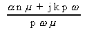 [9]
[9]
The distributed MCI application was then implemented on a cluster seven of DEC Alpha workstations. The goal of the original experiment [Dougherty 1994] was to demonstrate the impact of synchronization overhead. To accomplish this, the granularity of the problem was permitted to vary. Research by [Hummel et. al. 1992; Dougherty 1993] had shown that increasing the number of messages (implying an increase in Tcomm) could result in a decrease in synchronization penalty (Tsync). Timing Models were used to understand the interaction of the contributing issues for application performance.
Figure 6 below depicts the observed results as compared to those predicted by CTF graphs used in conjunction with Timing Models.
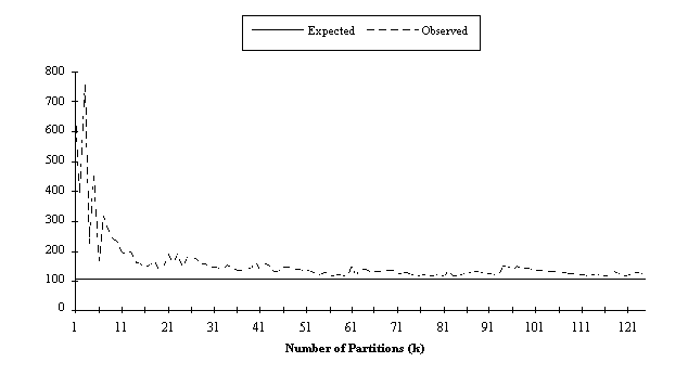 Figure
6: Expected and Observed Execution Times for MCI
Figure
6: Expected and Observed Execution Times for MCI
CTF graphs and Timing Models provide a better approximation
as the granularity is decreased (and the number of partitions
is increased). Application speedup and efficiency are given by
Speedup = = 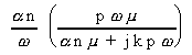 [10]
[10]
S =  [11]
[11]
S =
=  S=
S=
 =
=  [12]
[12]
Efficiency = = =  [13]
[13]
E =  [14]
[14]
E =
=  E=
0 [15]
E=
0 [15]
It is clear from [12] that the scalability of MCI is determined by the size of the problem, the speeds of the processor and the network, and the size of each message. Note that granularity (g) also influences the scalability of this application. For most practical problem, granularity is the most attractive parameter that the user can adjust to improve realized performance; the others are usually pre-determined by the topology available and the software that has been developed. However, it must also be noted that a larger value for granularity will introduce more dynamic synchronization overhead, an issue not accounted for in this model.
Results indicate that the maximum speedup realized for seven processors was 6.9987, with an efficiency of 99.98 %. However, from Figure 4 it is clear that the maximum is not always obtained; many studies [Hummel et. al. 1992] have investigated way to reduce this synchronization overhead. The significant result from Figure 4 is that CTF graphs, in conjunction with Timing Models, do identify a solid lower bound which can be used to evaluate a specific application for a given topology.
3.3.2 Steady-State Performability
From the previous section the following values were determined for distributed MCI: for seven processors, an expected execution time of T7 = 107.104 seconds, which is a speedup of 6.998 since the sequential applications needed Tseq = 749.6 seconds. This implies that the performance rate delivered to the end user was P7 = 42.5 mflop/second.
In this section other metrics are introduced to develop statistics for the expected performance and execution time considering partial failures and repairs. For this analysis, process availability is given as a = 0.98. For completeness sake, initially the study will assume that no fault tolerance is in place, implying that the application fails should any process fail.
Without fault tolerance, application availability
A = a11 = 0.80 [16]
and performability becomes
PA = P ï A = 34 mflop/second [17]
and the expected execution time is would be about 134 seconds.
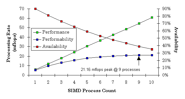
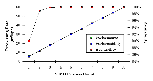
The graph in Figure 7 shows the relationship between performance, availability and performability for the SIMD component of the MCI application as the process count changes. To make this graph more illustrative, availability for a process was set at a = 0.9. As anticipated, performance increases while availability decreases. SSP, in conjunction with CTF graphs, provide the means to identify the point where delivered performance (i.e., performability) is maximized. The impact on designers (and budget personnel) of such a model is significant.
The analysis becomes significantly more interesting
when fault tolerance is introduced among the processes of the
SIMD element of the MCI CTF graph. Figure 8 below summarizes the
calculations needed for the SIMD element. There are eight states,
each corresponding to the number of worker processes executing
in that state. Time is measured in seconds, performance and performability
in flop/second.
| 107.10402 | 42482065.7 | 0.86812553 | 36879765.9 | |
| 124.951356 | 36414170.5 | 0.12401793 | 4516010.17 | |
| 149.937628 | 30345951.6 | 0.00759293 | 230414.829 | |
| 187.417035 | 24277409 | 0.00025826 | 6269.95854 | |
| 249.882713 | 18208542.5 | 5.2707E-06 | 95.9713135 | |
| 374.814069 | 12139352.2 | 6.4539E-08 | 0.7834602 | |
| 749.608138 | 6069838.05 | 4.3904E-10 | 0.0026649 | |
| _ | 0 | 1.28E-12 | 0 | |
| Application | Performability | 41632557.6 | ||
| Execution | Time | 109.289466 |
First looking at availability, the SIMD element results in availability near unity. When considered with the remaining processes of the application, MCI availability goes to
A = a4 ï [1 - (1-a)7] = 0.922 [18]
Figure 8 shows performability values for the SIMD component. Since the SIMD element is nested in the overall sequential CTF graph, the true performability becomes
PA = 38.4 mflop/second [19]
or about 118.5 seconds to execute.
One of the goals of SSP is to demonstrate quantitatively the benefits of fault tolerance. For MCI, delivered performance using fault tolerance among the processes of the SIMD construct results in an almost 13% increase in delivered performance.
Figure 9 below compliments Figure 7 to show the power of fault tolerance in realized performance. Again, as in Figure 7, availability is set to a = 0.9, and the underlying model has been modified to include the negative impact on performance of fault tolerant overhead. Still, the performability curve depicts the benefits of fault tolerance in this application. Figure 9 shows the scalability that fault tolerance adds to an application performance; in other words, the sky's the (theoretical) limit.
MCI is one of many distributed applications which can benefit from rigorous analysis using CTF graphs and decomposition tree traversal analysis methods. A representative sample of distributed applications is included as an appendix to this manuscript. A CTF graph is developed for each application in the survey; Timing Models and SSP then can be utilized as they were in this section for MCI.
4.0 SUMMARY AND FUTURE RESEARCH
This research supports CTF graphs as robust and complete tools for representing distributed applications across a wide spectrum. CTF graph construction, which implies problem decomposition, can be completed early in the design and implementation schedule. It has been noted that industry will not adopt any formalization unless benefits are realized immediately [Jackson and Wing 1996]; CTF graphs meet this criterion. The present work studies high-level CTF graphs before and after architecture issues are introduced. In the appendix, each of the 22 examples chosen has been modeled using the four CTF graph structures of sequential, pipeline, SIMD and MIMD, supporting the completeness of the CTF graphing approach.
The idea that a CTF graph can be used to represent any distributed application supported here is important because this graph is the starting point for such analysis as Timing Models and SSP, as well as proposed parallelizing compilers for distributed process [Shi 1993].
Another significant contribution of this work states that CTF is not only a possible way which can be used to build distributed applications, but that CTF is the proper technique to use. Other methods employ, in effect, trial and error, which is not deterministic. Deterministic techniques, such as chunking and PCAM, suggest decomposing the problem until it is realized that it has been decomposed too far, requiring agglomeration [Foster 1995]. CTF proposes a deterministic path to find the best way to decompose a target application for a target environment.
Research from this point will proceed to validate the proposed analytical tools. Previous work has demonstrated the usefulness of Timing Models [Shi and Blathras 1991; Dougherty 1994] and SSP [Dougherty 1995c; Dougherty 1995d]. Future research will unify these tools into a development approach for distributed applications which will handle the issues of performance, scalability, efficiency, and dependability [Dougherty 1995b].
5.0 REFERENCES
Aho, A.V., Hopcroft, J.E., and Ullman, J.D. Data Structures and Algorithms. Addison-Wesley, 1983.
Almasi, G.S., and Gottlieb, A. Highly Parallel Computing, second edition. New York: Benjamin Cummings, 1994.
Beetem, J., Denneau, M., and Weingarten, D. "The GF-11 parallel computer." in Dongarra, J.J., editor, Experimental Parallel Computing Architectures, Amsterdam: North-Holland, 1987.
Blathras, K. "A systematic dataflow realation method for computationally intense iterative algorithms." CIS Department (Preliminary Examination II), Temple University, April 1995.
Blathras, K., Szyld, D., and Shi, Y. "Parallel processing of linear systems using asynchronous methods." submitted to Supercomputing'96, Pittsburgh, PA, November 17 - 22, 1996.
Carriero, N. and Gelernter, D. "How to write parallel programs: a guide to the perplexed." ACM Computing Surveys, Vol. 21, No. 3, September 1989, pp. 323 - 359.
Cooley, J.W., and Tukey, J.W. "An algorithm for the machine calculation of complex Fourier seris." Math. Comp. 19(1965), pp. 297 - 301.
Dekel, E., Nassimi, D., and Sahni, S. "Parallel matrix and graph algorithms." SIAM Journal on Computing, Vol. 10, No. 4, November 1981, pp. 657 - 675.
Dougherty, J.P. "Variable-sized partitioning approaches for a distributed application." in Joint Conference on Information Sciences, November 1994, Pinehurst, NC.
Dougherty, J.P. "A performability model for parallel and distributed applications." Mid-Atlantic Workshop on Programming Languages and Systems, East Stroudsburg University, April 8, 1995, 8 pgs. [Dougherty 1995a]
Dougherty, J.P. "Prediction and evaluation of fault tolerant parallel and distributed applications." CIS Technical Report (Preliminary Examination II), Temple University, May 12, 1995, 41 pgs. [Dougherty 1995b]
Dougherty, J.P. "A performability model for a replicated worker application." Second International Conference on Computer Theory and Informatics, Wrightsville Beach, NC, September 28 - October 1, 1995. [Dougherty 1995c]
Dougherty, J.P. "Performability models for replicated workers." European Simulation Symposium 1995, Erlangen-Nuremberg, Germany, October 26 - 28, 1995. [Dougherty 1995d]
Dougherty, J.P. "A performability model for applications using checkpointing." CIS Technical Report, Temple University, February 1996, 20 pgs. (submitted to SRDS'96).
Ebeling, C. "All the right moves: A VLSI architecture for chess." Ph.D. Dissertation, Carnegie-Mellon University, Pittsburgh, PA, 1986.
Foster, I. Designing and Building Parallel Programs: Concepts and Tools for Parallel Software Engineering. New York, NY: Addison-Wesley, 1995.
Horowitz, E., and Zorat, A. "Divide-and-conquer for parallel processing." IEEE Transactions on Computers, Vol. C-32, No. 6, June 1983, pp. 582 - 585.
Hummel, S.F., Schonberg, E., and Flynn, L.E. "Factoring: a method for scheduling parallel loops." Communications of the ACM, Vol. 35, No. 8, August 1992, pp. 90 - 101.
Jackson, D. and Wing, J. "Lightweight formal methods." IEEE Computer, Vol. 29, No. 4, April 1996, pp. 21 - 22.
Korsh, J.F. Data Structures, Algorithms, and Program Style. Boston: PWS, 1986.
Lawler, E.L. et. al., editors. The Traveling Salesman Probklem: a Guided Tour of Combinatorial Optimization. Wiley, 1985.
Lewis, T.G. Foundations of Parallel Programming: A Machine-Independent Approach." Washington, DC: IEEE Computer Society Press, 1993.
Lewis, T.G. "Supercomputers ain't so super." IEEE Computer, Vol. 27, No. 11, November 1994, pp. 5 - 6.
Lewis, T.G. "The next 10,0002 years: Part I." IEEE Computer, Vol. 29, No. 4, April 1996, pp. 64 - 70.
Murman, S. personal correspondence and WWW publication, "Introduction to Computational Fluid Dynamics," (http://www.best.com/~smurman/cfd_intro/ns_eqns.html).
Nelson, P.A. "Parllel programming paradigms." Ph.D. dissertation, Computer Science Department, FR35, University of Washington (87-07-02), July 1987, 132 pgs.
Nelson, P.A., and Snyder, L. "Programming paradigms for nonshared memory parallel computers." in Jamieson, L., Gannon, D., and Douglas, R., editors, The Characteristics of Parallel Algorithms, Cambridge, MA: MIT Press, 1987, pp. 3 - 20.
Parhami, B. "Panel assesses SIMD's future." IEEE Computer, Vol. 28, No. 6, June 1995, pp. 89 - 91.
Pfister, G.F. "An introduction to the RP3." in Dongarra, J.J., editor, Experimental Parallel Computing Architectures, Amsterdam: North-Holland, 1987.
Pfister, G.F. In Search of Clusters: The Coming Battle in Lowly Parallel Computing. Englewood Cliffs, NJ: Prentice-Hall, 1995.
Press, W.H., Flannery, B.P., Teukolsky, S.A., and Vetterling, W.T. Numerical Recipes: the Art of Scientific Computing. New York: Cambridge University Press, 1987.
Sahner, R.A., and Trivedi, K.S. "Performance and reliability analysis using directed acyclic graphs." IEEE Transactions on Software Engineering, Vol. 14, No. 10, October 1987, pp. 1105 - 1114.
Shi, Y. "The SAG distributed processing model and its application in scientific visualization." Proceedings of SIAM International Conference on Scientific Parallel Processing, Houston, March, 1991.
Shi, Y. "Stateless C-compiler design." CIS Technical Report, Temple University, December 1993.
Shi, Y. "Timing Models: towards the scalability analysis of parallel programs." CIS Technical Report, Temple University, August 1994.
Shi, Y. "Articulating the power of parallelism using steady-state timing models." CIS Technical Report, Temple University, May 1995.
Shi, Y., and Blathras, K. "MT: a distributed interface for graphic programming using hetergeneous networked computers." Proceedings of National Conference on Graphics Applications, April 1991.
Strassen, V. "Gaussian elimination is not optimal." Numerische Mathematik, Vol. 13, pp. 354 - 365, 1969.
Valdes, J., Tarjan, R.E., and Lawler, E.L. "The recognition of series parallel digraphs." SIAM Journal of Computing, Vol. 11, No 2, May 1982, pp. 298 - 313.
APPENDIX: SURVEY OF DISTRIBUTED APPLICATIONS
A.1 Embarrassingly Parallel Applications
The term "embarrassingly parallel" was coined around the time of the Grand Challenge announcements. A pejorative term, the common feature of such an application is the lack of data dependencies, making problem partitioning direct. Other characteristics of these applications include large data volumes and low communication overheads, both of which can be used to generate linear performance speedups and efficiencies close to unity. Monte Carlo Integration (from the previous section) is an example of such an application.
At the same time, embarrassingly parallel applications do provide a very good starting point for research because the characteristics are finite in number and simple in complexity. New features (e.g., IPC mechanisms, fault tolerance techniques) are often implemented first with these applications until the "kinks" are eliminated.
A.1.1 Mandelbrot Fractal
Fractals have enjoyed popularity recently because
of the graphical applications for video production. One of the
most popular fractals is the Mandelbrot set, which exhibits recursively
regular patterns. They are attractive for distributed/parallel
processing because of the lack of any dependency relationship
between any of the points in the data domain. Using SAG, the CTF
graph for the Mandelbrot Fractal Application is given below in
Figure A1:
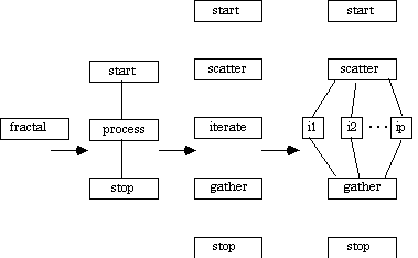
For this application, each step in the CTF graph development process has been pictured to show how the graph evolves to include the significant information needed at a high level. Initially the application is represented as a trivial single vertex. The next step uses sequential composition to detail the processing dependencies within the fractal application. In the third step, the process is specified in its constituent components of scatter, iterate, and gather; again, sequential composition is used. Finally, iterate is detailed using the simd composition rule, resulting the Fractal CTF graph.
In the remaining examples, only the non-trivial steps used in CTF graph development will be presented. It is understood that each example begins as a single node CTF graph.
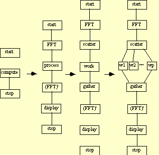
A.1.2 Ray Tracer
[Shi and Blathras 1991] have developed a distributed ray tracer application which decomposes the visual plane into columns which can be distributed among a set of processes, each of which computes at piece of an image. IPC is reduced by replicating the image components onto each processing element, and thus placing the application into the "embarrassingly-parallel category. The CTF graph for this ray tracer application is given below.
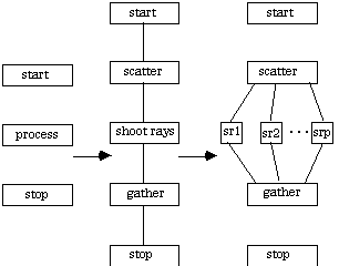
Each of the three applications in this section can be represented by similar CTF graphs. It is therefore reasonable that analysis for performance, execution time, availability and performability will also proceed in similar fashions.
A.1.3 VLSI Floorplan
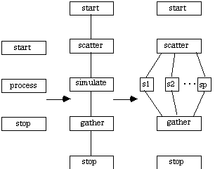
Parallelism is discovered in design automation for VLSI circuit manufacturing during the verification phase [Pfister 1987]. Simulation of the logic design is a probabilistic search for errors which is extremely complex and time-consuming for contemporary designs. Parallelism is found among the levels of logic in the hundreds of thousands of circuits in the processing unit. During a single (execution) cycle input bits cascade from one gate to the next until output bits are created. The good news is that this cascade usually falls into the range of 10 - 30 levels. This results in an average of about 10,000 gates per level which can be simulated in parallel.
Although special-purpose parallel processors (e.g., Yorktown Simulation Engine [Almasi and Gottlieb 1994]) have been constructed for VLSI simulations, a coarser approach can be envisioned. Consider a distributed VLSI simulation application which provides a copy of all the N gates of the VLSI floorplan to all P processes, and partitions the operations to be simulated among the processes using SAG implemented as SIMD. This would result in the CTF graph below.
A.2 Sorting Applications
These applications are seminal in computer science to the point where they warrant their own volume from Knuth. Distributed sorting applications involved extremely large amounts of problem data. Distributed searching applications exhibit large volumes of data and a substantial amount of computational density, which both contribute to the size of the problem.
A.2.1 Mergesort
This distributed application sorts the input set by splitting that set among the parallel processors available, sorting each subset, and then merging these subsets to form the sorted result. The CTF graph for Mergesort is generated as follows.
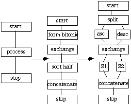
A.2.2 Bitonic Sort
[Lewis 1993] describes Bitonic Sort for a fine-grained parallel processing application (input size n = number of processors p). It is assumed that the application used in this context will be coarse-grained such that each processor will hold more than a single data item (i.e., n >> p). This divide and conquer algorithm is understood best using p = 2k processors.
Initially the data is rearranged such that half the data is in ascending order and the remaining half is in descending order. This is known as a bitonic sequence. To complete the sort, the fine-grained application divides the original bitonic sequence into two bitonic sequences, which is again divided until eventually the sequence is sorted. For this coarse-grained application, it is assumed that the original bitonic sequence is rearranged as in step 7 of Figure A5 below. Now the first half contains elements which are smaller than any elements in the other half. Each half is the sorted in parallel and simply concatenated. The CTF graph for Coarse Bitonic Sort is depicted in Figure A5.
A.2.3 Topological Sort
Given a directed acyclic graph G = (V, E), a topological sorting of this graph results in a list of all vertices in V such that if Vi is before Vj, then there exists no path from Vj to Vi. There are a number of parallel topological sorting algorithms referred to in [Nelson 1987]. The application presented here is implemented in two steps.
Each vertex Vi is assigned a level number Li. All source vertices (i.e., those with no incoming edges) are assigned a level number of zero. The remaining vertices are assigned a level number that is the length of the longest path from that vertex to any source vertex. Finally, the vertices are sorted into ascending order keying on level numbers, and thus producing a topological sorting of the original graph. This sorting of level numbers can be done using any sorting algorithm, including the previously described mergesort or bitonic sort [Nelson 1987].
The application described here is a coarser version of [Nelson and Snyder 1987] to reduce IPC traffic. Each node in the system receives a copy of the original graph, and is responsible for vertices, where P is the number of processors in the system. The level numbers for each vertex are assigned using either Floyd's of Dijkstra's algorithm to find the longest path. Once the level numbers have been set, the application sorts them, resulting in a topological sort of the original graph.
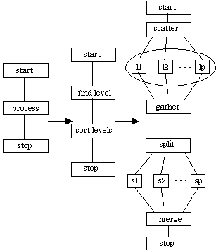
There are two SIMD components in the CTF graph for Topological Sort. The first SIMD component is enclosed in an ellipse to indicate that there is some IPC between these processes, but is quasi-synchronous and insignificant for this coarse analysis. Other applications will also exhibit this feature.
A.3 Searching Applications
A.3.1 All Pairs Shortest Path (APSP)
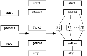
This applications searches for the shortest path between all pairs of vertices in a finite graph. Each edge in the graph is assigned a cost. If the graph is a digraph, then edge ij is distinct from edge eji, i_j. A path from vertex vi to vj is a sequence of edges where no edge appears more than once. The most popular solutions to this problem are Floyd's Algorithm and Dijkstra's Algorithm. Each will be expressed using CTF graphs.
A.3.1.1 Floyd's Algorithm
Sequentially, this algorithm is given in Figure 9 [Aho et. al. 1983]:
procedure sequential_floydbegin Iij(0) = 0 if i=j Iij(0) = length((vi, vj)) if edge exists and i_j Iij(0) = _ otherwise for k=0 to n-1 for i=0 to n-1 for j-0 to n-1 Iij(k+1) = min{Iij(k), Iik(k) + Ikj(k)} endfor endfor endfor S = I(n)end
[Foster 1995] suggests two ways to implement this algorithm in parallel. The first approach is based on a one-dimensional, row-wise domain decomposition of the matrix I and the output S. The following logic is usedfor k=0 to n-1 for i=low_i to high_i for j=0 to n-1 Iij(k+1) = min{Iij(k), Iik(k) + Ikj(k)};
At the kth step, each process requires the values of Ik1, Ik2, ... Ikn, implying that a broadcast of the entire row must be made. Assuming n³p, then each process must initiate at least one such broadcast. Such broadcasts can be made using hypercubes [Foster 1995], or can be made using other interprocess communication (IPC) mechanisms such as tuple space.
The CTF graph for Floyd's Algorithm is given below.
A.3.1.2 Dijkstra's Algorithm
This algorithm maintains a set of vertices T for which no shortest path has yet been found, and di as the shortest known path from vs to vi. Initially, T=V and di=_. The sequential version of Dijkstra's algorithm is given in Figure 13 [Foster 1995].procedure sequential_dijkstrabegin ds = 0 di = _ for i_s T = V for i=0 to n-1 find vm e T with minimum dm for each edge (vm, vt) with vt e T if (dt > dm + Lmt) then dt = dm + Lmt endfor T = T - vm endforend
Distributed Dijkstra's Algorithm is implemented by replicating the graph in each of the p processors. Each process executes the sequential algorithm for vertices. The corresponding CTF graph for Dijkstra is given here.
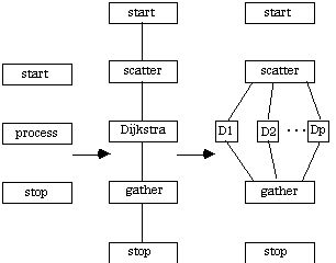
Figure A9 (Floyd) and Figure A11 (Dijkstra) are different applications, but from a coarse view they are equivalent.
It should also be noted that these APSP applications have been used in a parallel application for Topological Sorting [Dekel et. al. 1981].
A.3.2 Traveling Salesperson Problem (TSP)
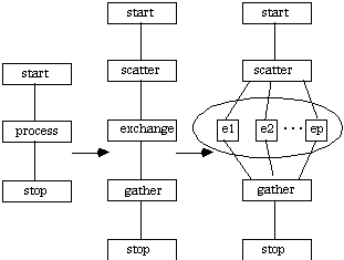
This is a fundamental application for computational complexity study. Given a graph, identify a tour of the vertices in this graph at minimal cost (i.e., traversing the set of edges incurring the minimal cost). A significant body of research exists on this problem [Lawler et. al. 1985], which is NP-hard. Parallel processing solutions have suffered due to IPC incurred [???]. A coarse-grained solution has been proposed by [Shi 1993] where the problem is viewed as a search through a tree. The initial level after the root is partitioned among the p processes. Each process searches its assigned subtree using branch and bound techniques. The CTF graph for this implementation of the TSP is given below.

A.4 Numerical Applications
A.4.1 Matrix Transposition
[Foster 1995] discusses two parallel algorithms for matrix transposition. The first one involves partitioning the matrix columnwise among the processes available. Given a two dimensional NxN matrix, each process would receive elements. It is expected that communication overhead would dominate this approach since it requires all-to-all IPC among the P processes. The amount of data to be exchanged between processes is . To reduce the number of exchanges, a hypercube algorithm is proposed which recursively exchanges data between pairs of processes. In a loosely-coupled environment it may be advisable to establish a lower threshold such that process sets simply exchange the appropriate data values.
Either algorithm can be implemented as a distributed application with the following CTF graph:
It should be noted that matrix transposition seems to exhibit a low computation/communication ratio, a characteristic which is usually indicative of slow performance for a distributed application.
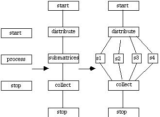
A.4.2 Matrix Multiplication
[Foster 1995] presents a set of parallel implementations for matrix multiplication, including one-dimensional columnwise decomposition, two-dimensional decomposition, and even a systolic solution. However, it is stated explicitly that these solutions are designed for situations where the number of processes P is not small [Foster 1995, p. 159]. Still, the analysis is of interest for it demonstrates the effect of different implementation approaches for the same application.
A matrix multiplication application based on Strassen's matrix decomposition [Strassen 1969] is given in [Nelson 1987]. Although this technique can be applied recursively, it is assumed here that the matrices are decomposed once. This implies that the matrix equation of NxN matrices AïB = C can be accomplished by decomposing each matrix into four submatrices of dimension x. This implementation assumes four processors. Either partitioning or replication of the submatrices can be used. Partitioning places a different submatrix from both A and B, and stores the corresponding resulting submatrix of C on the same processor. Replication places all of A and B on each processor, only a submatrix of C is computed by each processor. The choice between partitioning and replication is decided by IPC costs; partitioning generates 25% as much IPC as replication initially, but IPC during application execution can introduce communication and synchronization penalties. Replication eliminates these latter overheads.
The CTF graph for either implementation of matrix multiplication is given below.
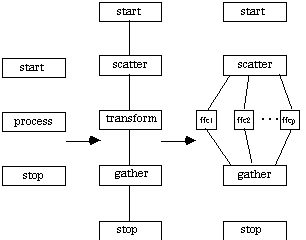
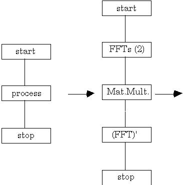
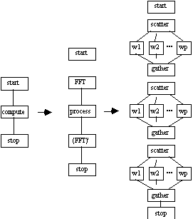
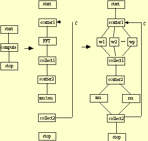
A.4.3 Fast Fourier Transform
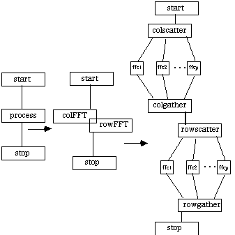
Fourier transform methods are used to take a function from the time, domain into the frequency domain where analysis is often more efficient [Press et. al. 1987]. Direct Fourier transformation is an O(N2) algorithm; the Fast Fourier Transform (FFT) accomplishes the same in O(N log N) [Cooley and Tukey 1965]. Also attractive is that FFT maps well into a parallel processing environment [Nelson 1987]. Assuming that the number of processors P and the input size N are each powers of 2 (as in [Press et. al. 1987]), then each processor is responsible for elements. Partitioning or replication can be used as in matrix multiplication, depending on the expected overheads. The CTF graph for this distributed application is given below.
A very interesting alternative is described in [Foster 1995] involving pipelining for a two-dimensional FFT used in image processing. A two-stage pipe is established, with processors in each stage. A one-dimensional column FFT is performed on an image, which is then sent to the next stage for a one-dimensional row FFT. In this way there are always two images in the pipe being transformed. The CTF graph for this implementation is give below.
A.4.4 Convolution
Convolution is the operation which allows us to find the output of a linear time-invariant system given the input and the impulse response. Assuming a linear (time-invariant) system whose impulse response is given by h(t), then the input function, x(t) can be expressed as a weighted sum of an infinite number of shifted impulses. Now, the output for an input of d(t) is simply h(t) by definition of the impulse response. Similarly, since the system is shift invariant, the output for an input of d(t-t) is h(t-t) since the system is time-invariant. Lastly, since the system is homogeneous, scaling the input will simply result in scaling the output, and since the system is additive, the contribution to the individual impulses can be simply summed (or integrated) together. Therefore, the output of a linear time-invariant system with input signal x(t) and impulse response h(t) is given by
This relationship between input, impulse response, and output of the system is known as convolution. Convolution is often denoted using the notation
which is linear and time-invariant.
A discrete, linear and shift-invariant system can be described in terms of linear difference equations with constant coefficients. That is, we are interested in obtaining the input/output relationship. If we apply transform methods, like the Fourier transform, a system can be described in terms of algebraic equations. Another method of describing a system is via discrete convolution. There is also a very important connection between convolution and transform methods. Utilizing the Fourier transform, the theorem states that the convolution of two functions in one domain is equivalent to multiplication in the second domain and vice versa [Press et. al. 1987].
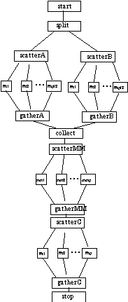
From the above discussion, it is clear that a distributed convolution application can be built from existing FFT and matrix multiplication applications. The CTF graph for such an application is given here.
A.5 Scientific Applications
A.5.1 Weather Codes
This application, also known as Atmosphere Modeling [Foster 1995], simulates atmospheric processes, (e.g., wind, clouds, precipitation) that influence weather or climate. This is accomplished by solving a set of partial differential equations which describe the fluid dynamics of the atmosphere. The application performs a time integration to determine the state of the atmosphere at some future time based on an initial state. The atmosphere is modeled as a three-dimensional volume with axes of longitude, latitude, and altitude (the poles are ignored).
For this example, the equations used for humidity will be discussed, similar to [Almasi and Gottlieb 1994]. The state of the atmosphere is characterized by the following quantities:
V = (u, v) horizontal components of wind velocity
T temperature
q specific humidity
p shifted surface pressure
f geopotential
s vertical component of wind velocity
p pressure
The sequential algorithm for these humidity equations are given below [Almasi and Gottlieb 1994].ForEach longitude, latitude, altitude u*[i, j, k] = n * (p[i, j]) * (u[i, j, k]) v*[i, j, k] = m[j] * (p[i, j]) * (v[i, j, k]) S*[i, j, k] = p[i, j] * (s*[i, j])EndForEach longitude, latitude, altitude D = 4 * ((u*[i, j, k] + u*[i-1, j, k]) * (q[i, j, k] + q[i-1, j, k]) ... terms for i±1, i±2, j±1, j±2, k±1) pq[i, j, k] = pq[i, j, k] + D * Dt ï four similar of statements for pu, pv, pT, and p ï ïEndForEach longitude, latitude, altitude q[i, j, k] = pq[i, j, k] / p[i, j, k] u[i, j, k] = pu[i, j, k] / p[i, j, k] v[i, j, k] = pv[i, j, k] / p[i, j, k] T[i, j, k] = pT[i, j, k] / p[i, j, k]End.
The distributed application to determine these humidity equations should exploit the following observations. Statements within each of the above three ForEach loops can be executed concurrently; synchronization is needed only at the end of each loop. The CTF graph in the following figure depicts the distributed application for weather codes.
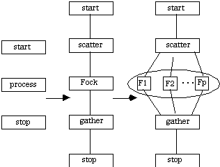
A.5.2 Computational Chemistry (Fock Matrix)
Formally known as ab initio quantum chemistry, computer applications are utilized to compute bond strengths and reactions energies (from first principles) for atoms and molecules by solving various approximations to the Schrodinger equation. A seminal structure used in quantum chemistry is the Fock matrix (F), a two-dimensional array which captures the electronic structure of an atom or molecule. Each element requires 2N2 integrals, implying the total computational work to be 2N4; in practice, redundancy can be used to reduce the amount of computation to about . The algorithm for Fock matrix construction is given below.procedure fockbegin for i = 1 to N for j = 1 to i for k = 1 to j for l = 1 to k integral (i, j, k, l) endfor endfor endfor endforendprocedure integral (i, j, k, l)begin I = computer_integral (i, j, k, l) Fij = Fij + Dkl I Fkl = Fkl + Dij I Fik = Fik + Djl I Fjl = Fjl - Dik I Fil = Fil - Djk I Fjk = Fjk - Dil Iend
[Foster 1995] suggests a parallel implementation involving functional decomposition which partitions the resulting elements of the matrix F among processes. The most difficult obstacle to overcome is the irregular access pattern to the D and F matrices. The suggested implementation avoids total replication due to issues of scalability in favor of a partial replication approach exploiting row-column locality to reduce IPC overhead.
The distributed application suggested here utilizes total replication among the P processes. In [Foster 1995], scalability is an issue due to the assumption of 16 MB memory per processor on a 512-processor multiprocessor. A more coarse-grained, multicomputer environment is assumed here where greater than 16 MB of memory per processor is reasonable. At the same time, one can argue that even if the 16 MB restriction is maintained, virtual memory would still be faster than IPC, again supporting total replication.
Using total replication, the CTF graph for the construction of the F matrix is a scatter and gather is given below.
A.5.3 Seismic Migration
The discussion for this application is taken primarily from [Almasi and Gottlieb 1994]; however, they use a manager - worker implementation, which differs from the implementation assumed in the present context.
Seismologists use seismic migration to obtain an undistorted subsurface image from seismic echo data for many applications in the petroleum industry. The main difficulty with this type of image processing is that propagation velocities of signals can vary by factors of ten. The methodology used involves solution of the sonic wave equation run backward in time. Using finite differences, the wave equation
ó2P =
using a Fourier Transform to the frequency domain w. This is followed by a downward extrapolation at each frequency which resembles convolution. The output is an array in which each (x, z) entry is the sum over all ws of the computed (x, z, w) values.
Concurrency exists among the frequency values (w). Using Scatter and Gather (SAG), implemented as SIMD, the following CTF graph is generated
A.5.4 Synchronous Apture Radar (SAR)
SAR is an image processing problem involving a stream of input images which must be analyzed. This analysis may imply a search for pre-determined objects or patterns in the image stream, as well as the size, number, direction, and velocity of these objects. Parallelism exists explicitly in the constituent analysis modules employed, such as FFT, matrix multiplication, and convolution. At the same time, parallelism is implied by the stream of input which forms a pipeline, overlapping different stages as they work on distinct images in the stream. The CTF graph for SAR is given below.
A.6 Coarsely-Iterative Applications
A.6.1 Magnetic Fields
This application is seminal because it involves the iterative solution of a linear system, a methodology employed in a variety of scientific fields. The magnetic field application studied here uses a novel approach of trading computation for communication to improve performance in a distributed environment.
The objective is to determine the magnetic field in a region outside of a permanent magnet. By choosing the two-dimensional form of the problem for a magnet of rectangular geometry that is uniformly magnetized, the equation can be solved in its Laplacian form
+ = 0
Using Taylor's expansion to obtain a finite difference equation results in the expression
fi,j(t + 1) =
This Jacobi scheme is accelerated via Gauss-Seidel, which uses new values as soon as they are available
fi,j(t + 1) =
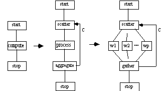
These grid points are partitioned among a set of processes as in SAG; however, there is a data dependency points within along the boundaries of adjacent partitions which mandates IPC. Once intermediate data has been exchanged processing resumes. Convergence is also detected during this exchange phase. A novel application, called an Asynchronous Linear System Solver (ALSS), is proposed in [Blathras et. al. 1996].
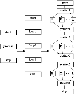
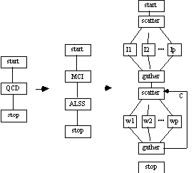
Applications of this type have been classified as Compute-Aggregate-Broadcast, or CAB [Nelson 1987]. In the CTF graph below, a cycle is introduced. The cycle count C is fixed and is determined in practice by the rate of convergence of the application.
A.6.2 Quantum Chromodynamics (QCD)
Quantum Chromodynamics (QCD) is a theory involving hadrons, the particles that make up atomic nuclei. Hadrons include protons, neutrons, delta baryons, pions and others. QCD proposes that there are even more elementary particles called quarks and antiquarks bound together by the chromoelectric field. Motion of a quark through this field is partly random, as is the field itself. Using transition probabilities, relatively simple formulas can be derived; for example, the mass of a proton can be obtained from transition probabilities of a system of three quarks which comprise the proton.
The details of QCD computations are sketched here so that a CTF graph can be generated. The space-time continuum is approximated by an NxNxNxN four-dimensional lattice. The quark field f at each lattice site is a 12-element complex vector, implying 24 variables per lattice site. The chromoelectric field U at each link in the lattice is a 3x3 complex matrix, and four links per site must be considered, but only eight matrix elements are independent, implying 32 more variables per site for a total of 56 variable per lattice site. The probability of a transition is expressed as an integral depending on these two fields as well as the transition in question [Almasi and Gottlieb 1994].
Even for small values of N = 8, deterministic methods of numerical integration would require astronomical amounts of time. In this situation, Monte Carlo Integration (see ???) is used [Beetem et. al. 1987]. A random sequence of lattice configurations of the U and f variables are generated, and the corresponding functions are evaluated for each configuration, with values averaged to produce approximations for the transition probabilities. Generation of each new configuration involves a matrix equation which needs to be solved. The total number of operations where N = 24 is about 1017, which at 10 GFLOPS requires about 100 days [Almasi and Gottlieb 1994].
Parallelism for such a QCD application is found in the Monte Carlo Integration used to approximate the transition probability, as well as the matrix equations. The CTF graph for the QCD application is given below.
A.6.3 Navier-Stokes (N-S)
The Navier-Stokes Equations are a set of partial differential equations that represent the equations of motion governing a fluid continuum (i.e., a viscous fluid). The set contains five equations; namely mass conservation, three components of momentum conservation, and energy conservation. In addition, certain properties of the fluid being modeled, such as the equation of state, must be specified. The equations themselves can be classified as non-linear and coupled. Non-linear, for practical purposes, means that solutions to the equations cannot be added together to get solutions to a different problem (i.e., solutions cannot be superimposed). Coupled means that each equation in the set of five depends upon the others, so that they must all be solved simultaneously. If the fluid can be treated as incompressible, then the conservation of energy equation can be decoupled from the others and a set of only four equations must be solved.
The Navier-Stokes Equations model the majority of fluid dynamics flows. Though a common misconception, these equations are also the governing equations for turbulent flows. It is generally agreed that turbulence is modeled by the Navier-Stokes Equations; however, the many scales of motion that turbulence contains cause the modeling of turbulent processes to require an extremely large number (i.e., high density) of grid points. These simulations are termed Direct Navier-Stokes Simulations (DNS). These DNS simulations are currently only able to model a very small region, in the range of 1 sq. ft., using current supercomputers [Murman 1996].
A distributed Navier-Stokes application has been proposed in [Lui 1996] which utilizes both SIMD and MIMD parallelism. The CTF graph for this application is given below.
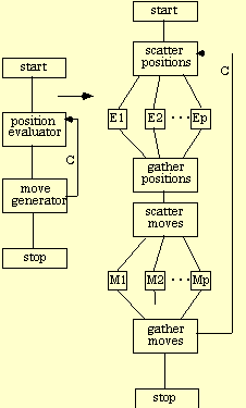
A.6.4 Ebeling's HiTech Chess
This application utilizes a custom VLSI architecture and parallelism for move generation and position evaluation [Ebeling 1986]. However, it is possible to envision a distributed implementation of this application. The following CTF graph in Figure A27 depicts the HiTech Chess application.