Example: Given the following matrix dimensions:
A1 is 30-by-35
A2 is 35-by-15
A3 is 15-by-5
A4 is 5-by-10
A5 is 10-by-20
A6 is 20-by-25
Dynamic Programming and Memoization
Example: Fibonacci numbers
Direct recursive algorithm:
    Fibonacci-R(n)
    1  if n < 2
    2      then return n
    3  return Fibonacci-R(n-1) + Fibonacci-R(n-2)
Complexity: Θ(φn), φ ∼ 1.618 ("golden ratio").
Repeated work: to calculate F(4), the algorithm calculates F(3) and F(2) separately though in calculating F(3), F(2) is already calculated.
Dynamic programming: to turn a "top-down" recursion into a "bottom-up" construction.
    Fibonacci-DP(n)
    1  A[0] <- 0        // assume 0 is a valid index
    2  A[1] <- 1
    3  for j <- 2 to n
    4      A[j] <- A[j-1] + A[j-2]
    5  return A[n]
Complexity: Θ(n).
Memoization: a variation of dynamic programming that keeps the efficiency, while maintaining a top-down strategy.
    Fibonacci-M(n)
    1  A[0] <- 0        // assume 0 is a valid index
    2  A[1] <- 1
    3  for j <- 2 to n
    4      A[j] <- -1
    5  Fibonacci-M2(A, n)

    Fibonacci-M2(A, n)
    1  if A[n] < 0
    2      then A[n] <- Fibonacci-M2(A, n-1) + Fibonacci-M2(A, n-2)
    3  return A[n]
Complexity: also Θ(n).
Dynamic programming used in optimization: the optimal solution corresponds to a special way to divide the problem into sub-problems. When different ways of division are compared, it is quite common that some sub-problems are involved in multiple times. The complexity of such a solution comes from the need of keeping intermediate results, as well as remembering the structure of the optimal solution, i.e., how the problem is divided into sub-problems, step by step.
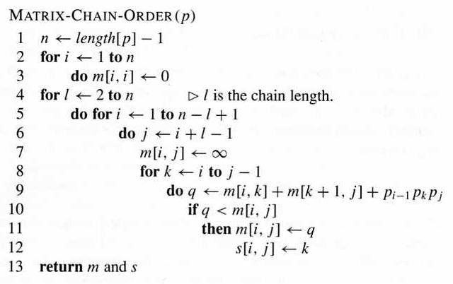
To calculate the product of a matrix-chain A1A2...An, n-1 matrix multiplications are needed, though different orders have different costs.
For matrix-chain A1A2A3, if the three have sizes 10-by-2, 2-by-20, and 20-by-5, respectively, then the cost of (A1A2)A3 is 10*2*20 + 10*20*5 = 1400, while the cost of A1(A2A3) is 2*20*5 + 10*2*5 = 300.
For matrix-chain Ai...Aj where each Ak has dimensions Pk-1-by-Pk, the minimum cost of the product m[i,j] corresponds to the best way to cut it into Ai...Ak and Ak+1...Aj:
    m[i, j] = 0                                         if i = j
              min{ m[i,k] + m[k+1,j] + Pi-1PkPj }        if i < j
Use dynamic programming to solve this problem: calculating m for sub-chains with increasing length, and using another matrix s to keep the cutting point k for each m[i,j].
Example: Given the following matrix dimensions:
A1 is 30-by-35
A2 is 35-by-15
A3 is 15-by-5
A4 is 5-by-10
A5 is 10-by-20
A6 is 20-by-25
then the output of the program is
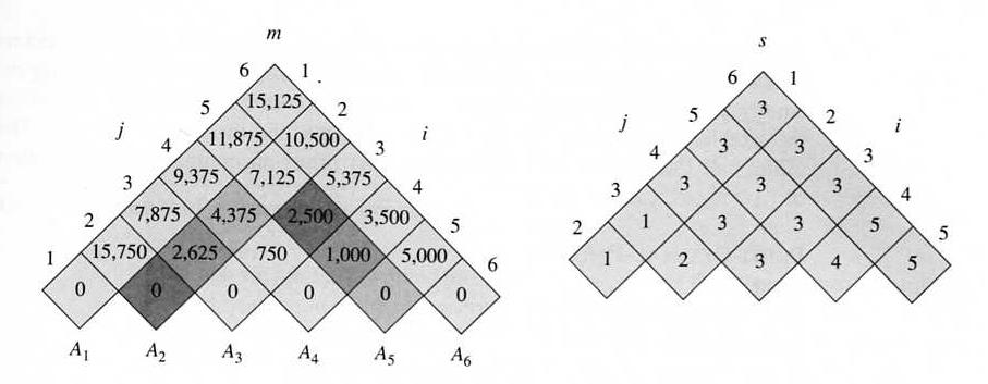
which means that A1A2A3A4A5A6 should be calculated as (A1(A2A3))((A4A5)A6), and the number of scalar multiplication is 15,125.
Time cost: Θ(n3), space cost: Θ(n2).
Please note that this algorithm determines the best order to carry out the matrix multiplications, without doing the multiplications themselves.
For sequence X and Y, their LCS can be recursively constructed:
c[i,j] = 0                         if i == 0 or j == 0
         c[i-1,j-1]+1              if i,j>0 and Xi == Yj
         max(c[i,j-1],c[i-1,j])    if i,j>0 and Xi != Yj
Time cost: Θ(mn). Space cost: Θ(mn).
Demo applet.
(2) Optimal Binary Search Tree
If the keys in a BST have different probabilities to be searched, then a balanced tree may not give the lowest average cost (though it gives the lowest worst cost). Using dynamic programming, BST with optimal average search time can be built, in a way similar to matrix-chain multiplication.
Time cost: Θ(n3). Space cost: Θ(n2). Demo applet.