Self-balancing BST
Since in a Binary Search Tree (BST) all major operations have worst-case costs proportional to the height of the tree (i.e., the number of edges on the longest path from the root to a leaf), a "balanced" BST will be close to the best case, in which each node has two subtrees with similar heights. However, to keep this balance, structure adjustments are needed after certain insertions and deletions. Self-balancing BSTs have this capability, though they achieve it in different ways.
Let's start with BSTs with 3 nodes, A, B, and C. Depending on their order of insertaion, the BST has 5 possible shapes, but only one of the them is balanced.
In the following case, each node shows its key over its balance factor
                C/2
                /
              B/1
              /
            A/0
This is considered a "LL" situation, as the unbalanced node C is "left heavy" (+2) and so is its left child B (+1).
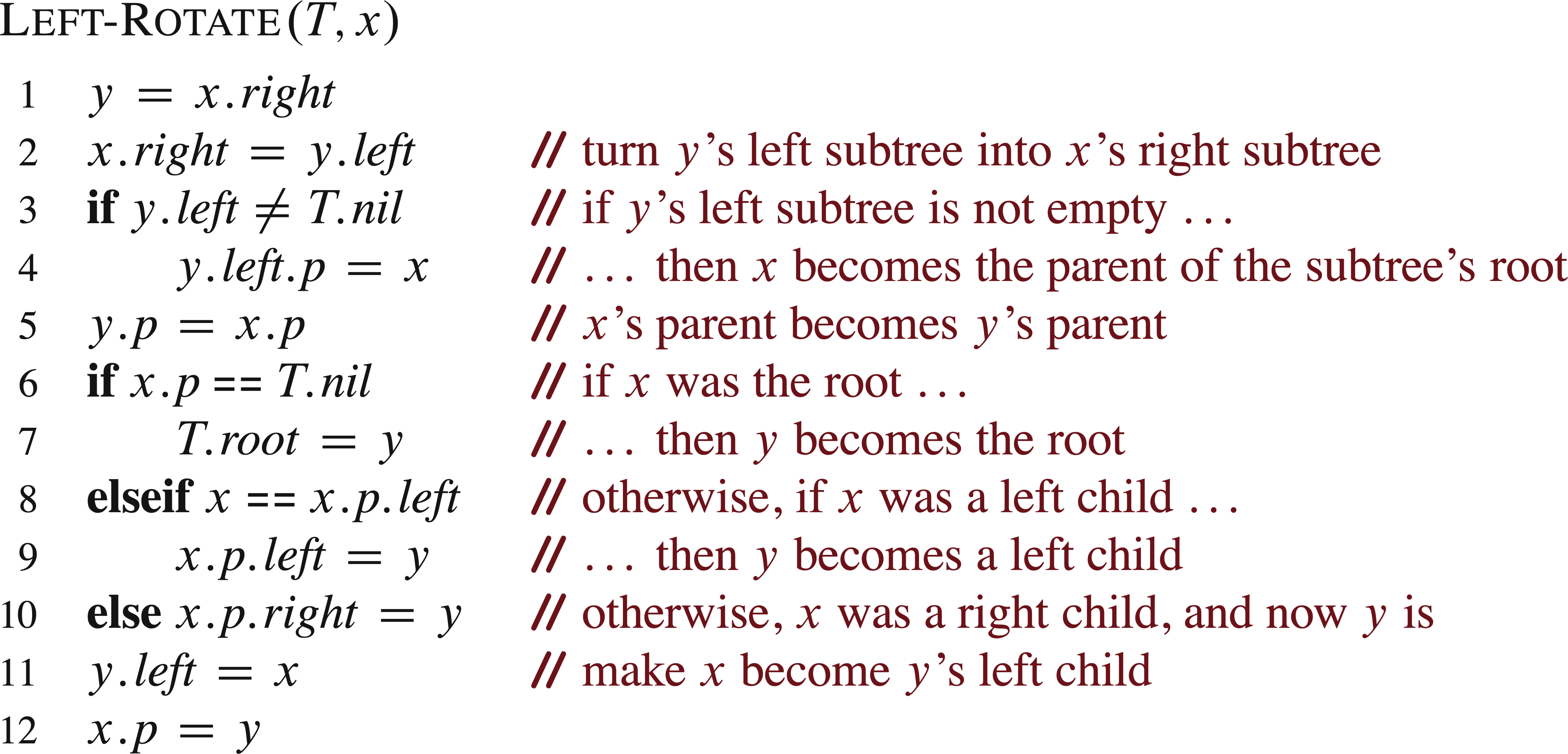
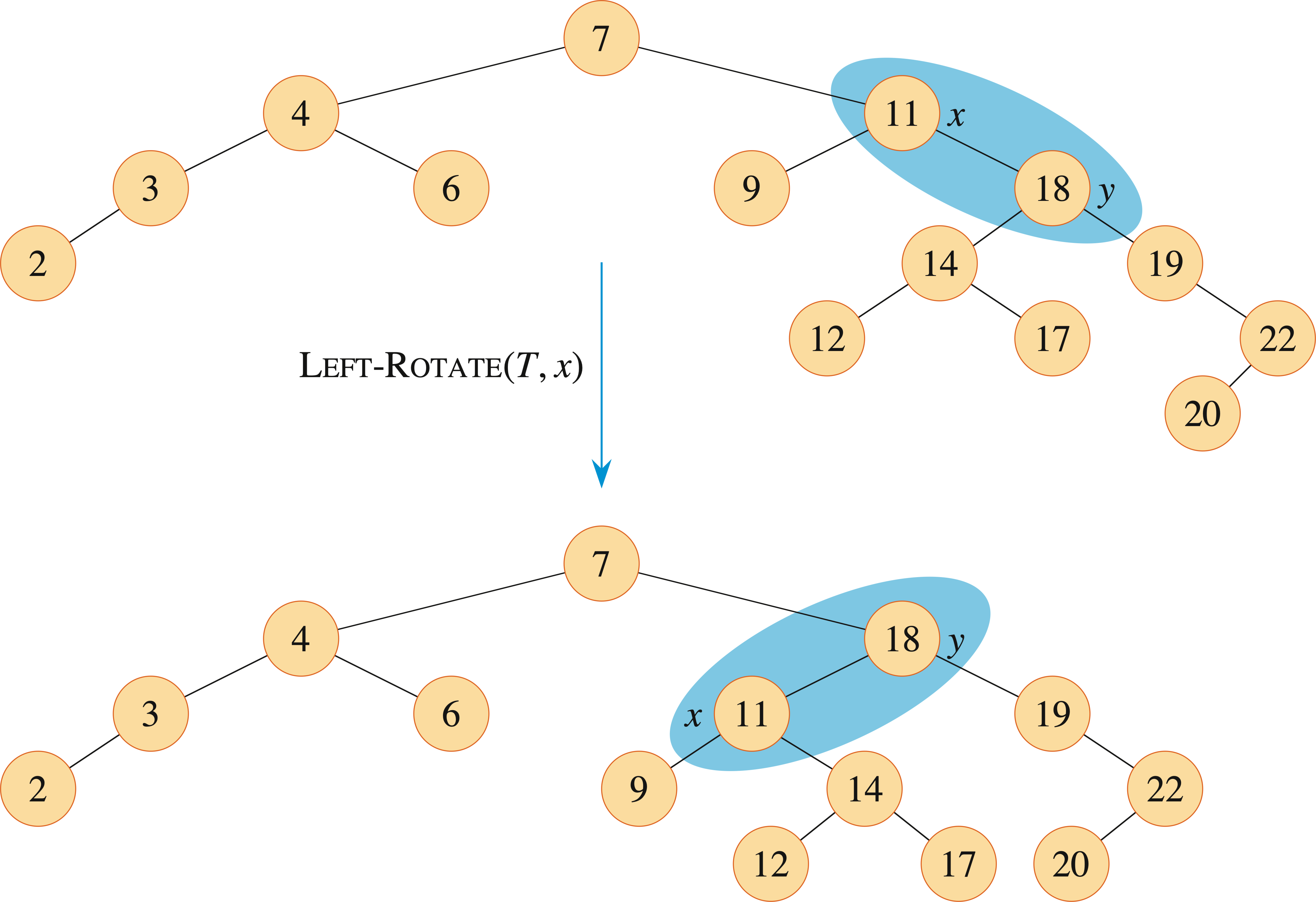
To rebalance the tree without changing the relative order of nodes (as defined in BST), a rotation is used.
The result of a right rotation of the top 2 nodes leads to
           B/0
          /  \
        A/0  C/0
Another case:
            C/2
            /
          A/-1
           \
           B/0
This is a "LR" situation, as the unbalanced node C is "left heavy" (+2), and its left child A is "right heavy" (-1). After a left rotation of the bottom 2 nodes:
            C/2
            /
          B/1
          /
        A/0
which is the "LL" case, then after a right rotation the tree is balanced
           B/0
          /  \
        A/0  C/0
There are two mirror-image cases: "RR" and "RL".
The above process can be extended into general situations in BSTs (not limited to AVL trees). In such a situation, a rebalancing is still achieved by rotations, which change certain balance factors, while keeping the order of all the nodes involved.


The algorithm is used in the following BST:

After an insertion or deletion in an AVL tree, one or more "out-of-balance" nodes (with balance factor 2 or -2) may appear in the path from the root to the insertion/deletion location, but cannot occur outside the path. If we check the "out-of-balance" node that is the "deepest" (the farthest from the root), there are only 4 canonical forms.
LL case:
              C/2
             /   \
          B/1     CR
         /   \
      A/0     BR
     /   \
   AL     AR
Here subtrees AL, AR, BR, and CR have the same height.
By the definition of BST, the order among the keys satisfy AL < A < AR < B < BR < C < CR
This requires a right rotation. B will become the root of the (local) tree. Its right subtree will be C. C will no longer have B as the root of its right subtree but will have BL instead. B and C have balance factors of 0. The balance factors of the other nodes remain the same as before.
          B/0
         /   \
      A/0     C/0
     /  \    /   \
   AL    AR  BR   CR
where we still have the order AL < A < AR < B < BR < C < CR.
LR Case:
               C/2
              /   \
          A/-1     CR
         /    \
       AL     B/0
             /   \
            BL    BR
Assume that all the subtrees, AL, BL, BR, and CR, have the same height. For the order among the nodes, here we have
AL < A < BL < B < BR < C < CR.
A left rotation at A:
              C/2
             /   \
          B/1     CR
         /   \
       A/0    BR
      /   \
     AL    BL
then a right rotation at C:
          B/0
         /   \
      A/0     C/0
     /   \   /   \
    AL    BL BR   CR
where we still have AL < A < BL < B < BR < C < CR.
The RL and RR cases are symmetric.
These four cases cover all possibilities. For the deepest out-of-balance node (i.e., with balance factor 2 or -2), if its child on the heavy side has balance factor 1 or -1, it directly maps into one of the above four cases: 2/1 to LL, 2/-1 to LR, -2/-1 to RR, and -2/1 to RL. If the third node (A in LL, B in LR and RL, and C in RR) has a balance factor 1 or -1, we can still use the above procedure to rebalance the tree. If the heavy-side child has balance factor 0 (which can only happen after a deletion, but not after an insertion), it is treated as LL or RR, and the tree will be balanced properly.
An AVL tree is maintained by making some changes to the algorithms for BST insertion and deletion. We can visualize the change as updating the balance factor of nodes along the path from the insertion/deletion position to the root and rebalance it if a +2 or -2 is found.
In a balanced BST, the time complexity of search, insertion, and deletion is O(log n), so it is usually more efficient than BSTs and linear data structures (array and linked list, sorted or not) in the major operations.

In a Red-Black tree, A node is either black (regular) or red (extra). The tree has the following properties:
Similar to in AVL tree, an insertion in a Red-Black tree is an insertion in a BST, sometimes followed by a rotation to keep the balance, plus the re-coloring of certain nodes to keep the above properties. The rebalancing algorithm is much more complicated than the one for AVL tree.
In a Red-Black tree, the major operations take O(log N) time in the worst cases, as in an AVL tree. However, since in Red-Black trees the notion of "balance" allows more shapes than in AVL trees, rotations happen less often, so it is considered more efficient.
The Java TreeMap class is based on a Red-Black tree.


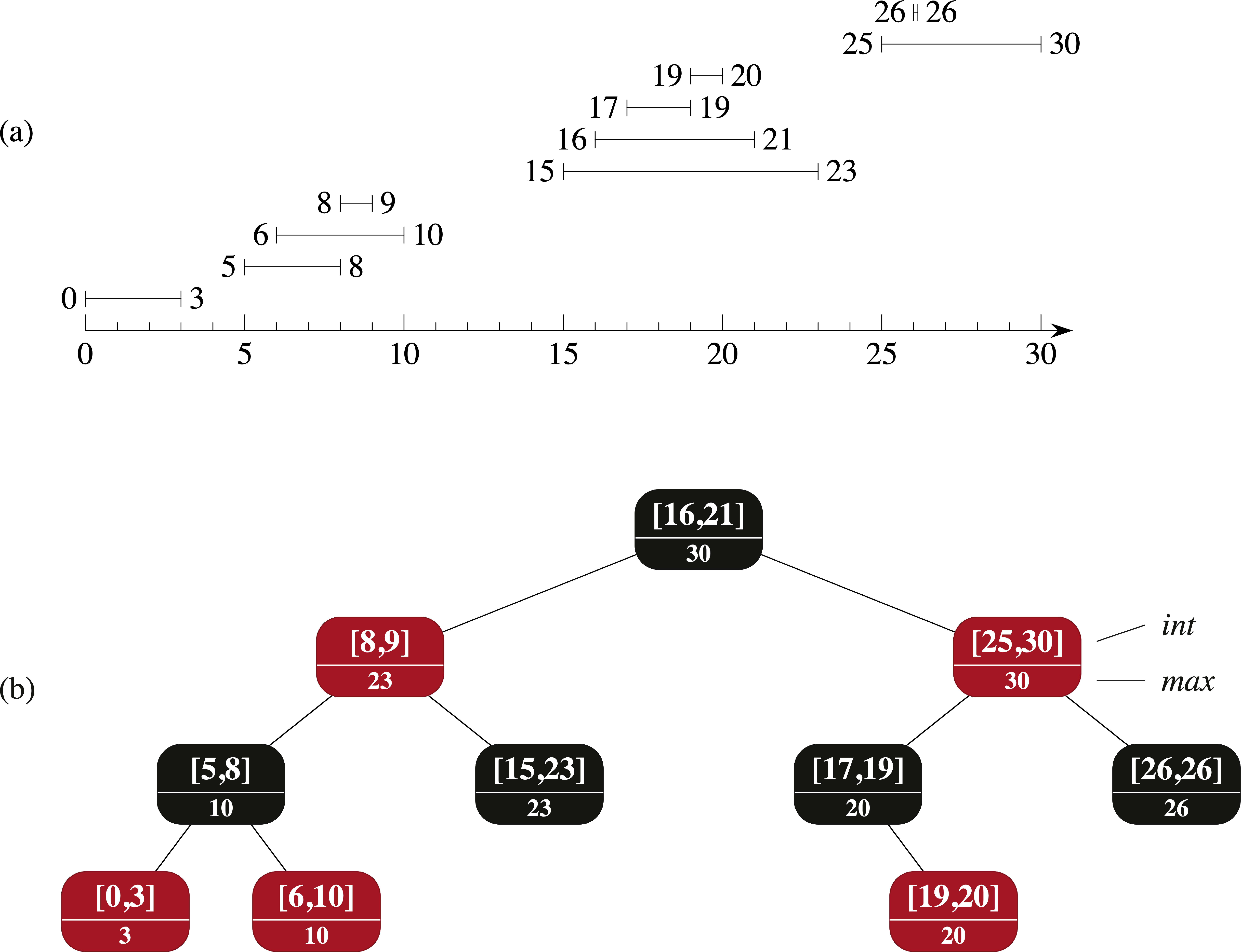
Red-black trees can also be augmented to support operations on dynamic sets of intervals, which can be open or closed. The key of each interval x is the low endpoint, x.int.low, of the interval. In addition to the intervals themselves, each node x contains a value x.max, which is the maximum value of all interval endpoints stored in the subtree rooted at x.
 Algorithm INTERVAL-SEARCH(T, i) searches the tree T for the given interval i, and use the additional information max to decide if a subtree should be searched.
