Sorting (2)
The (Lomuto) partition algorithm separates the elements of array A between index p and r that are smaller than the pivot value from the elements larger than it.
Example of partition:
Loop invariant:
Hoare partition let two index values start at the two ends of the array, then move toward each other. In the process, a pair of elements are exchanged into their corresponding regions. The following algorithm uses the first element as the pivot and returns the index j such that elements in A[p..j] are not larger than elements in A[j+1..r]:
The best case of Quicksort has T(n) ≤ 2T(n/2) + Θ(n) = O(n lg n). The result is the same even if the partition is uneven, where T(n) = T(n/a) + T(n(1 − 1/a)) + Θ(n) = O(n logan) = O(n lg n).
The worst case of quicksort happens when the pivot values are always at the end of the array --- in that case it becomes selection sort, and the running time is T(n) = T(n − 1) + Θ(n) = Θ(n2). A worst case is when the input is already sorted. To prevent the worst-case from consistently happening, pivot values can be randomly picked, or selected from a small number of elements (e.g., using indices 1, n/2, n).
In average case, when the partitions are sometimes good and sometimes bad, the expected running time will be closer to the best-case than to the worst case, so this algorithm is usually considered as O(n lg n).
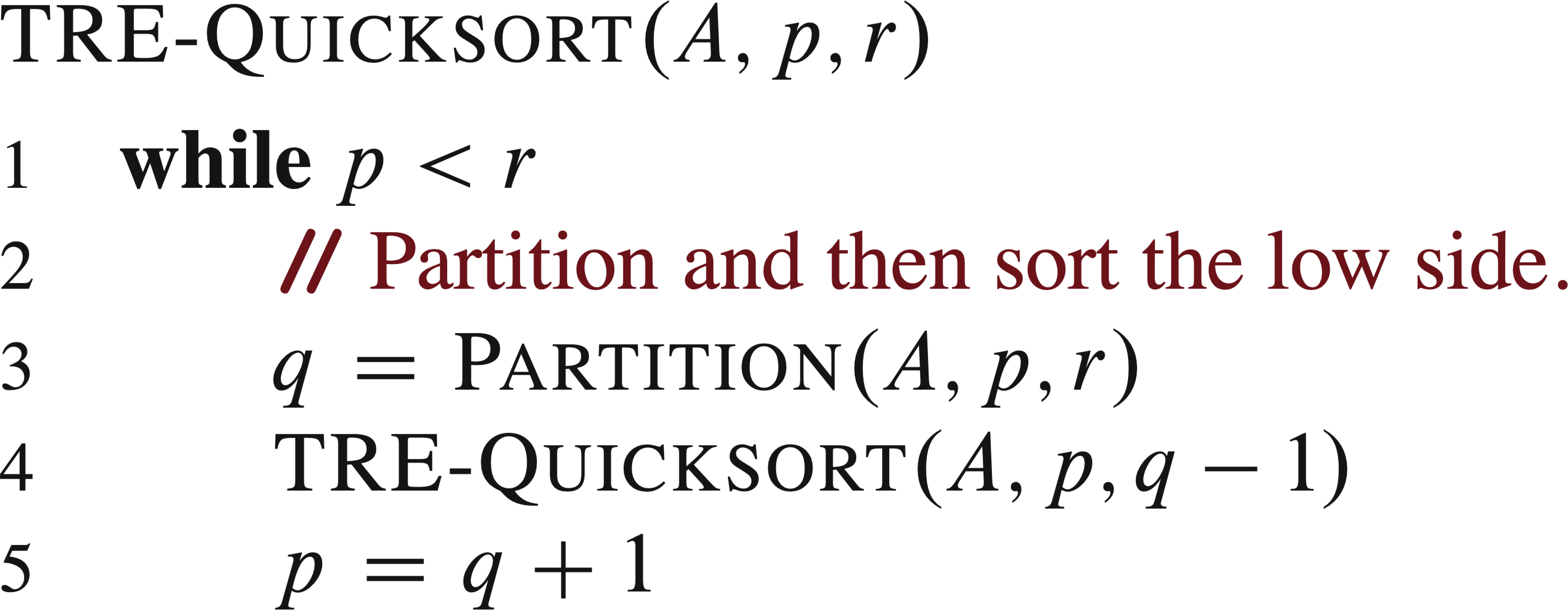
To reduce the overhead of recursion, the second recursive call in Quicksort can be replaced by an iteration:
The major comparison sorting algorithms are summarized in the following table in their recursive forms, with time function T(n) = D(n) + a*T(f(n)) + C(n):
| sort(first, last) | Linear: 1 * T(n − 1) | Binary: 2 * T(n / 2) |
| with preprocessing D(n) = O(n) C(n) = O(1) |
SelectionSort
select(last); sort(first, last − 1); | QuickSort
partition(first, last); sort(first, middle − 1); sort(middle+1, last); |
| with post-processing D(n) = O(1) C(n) = O(n) |
InsertionSort
sort(first, last − 1); insert(last); | MergeSort
sort(first, middle); sort(middle+1, last); merge(first, middle, last); |
For a sorting problem with n different items, there are n! possible input, in terms of the relative order of the items (here the actual values of items does not matter), and each needs a different processing path. Therefore it is enough to analyze an array containing integers 1 to n. Comparison sorts can be viewed in terms of decision trees to distinguish the cases. If we see each comparison as a node, then a sequence of comparisons forms a binary tree. The execution of an algorithm corresponding to a path from the root to a leaf, and each leaf corresponds to a different execution path for a specific order.
The decision tree corresponding to a (comparison-based) sorting algorithm must have n! leaves to distinguish all possible inputs, and the worst case corresponds to the longest path from the root to a leaf. Since a binary tree of height h has no more than 2h leaves, we have n! ≤ 2h, that is, lg n! ≤ h, while the former is Θ(n lg n) (see Page 67, Equation 3.28). Therefore, h = Ω(n lg n).
This result gives us a lower bound of the comparison-based sorting problem, independent of the algorithm used to solve the problem.
As for the best case, it is easy to see that each item must be compared at least once, so the lower bound is Ω(n), which is also the lower bound of the average case.