Dynamic programming
Example: Fibonacci numbers
Direct recursive algorithm:
    Fibonacci-R(n)
      if n < 2
          then return n
      return Fibonacci-R(n-1) + Fibonacci-R(n-2)
Complexity: T(n) = T(n – 1) + T(n – 2) + Θ(1) = Θ(φn), φ ∼ 1.618 ("golden ratio").
Repeated work: to calculate F(4), the algorithm calculates F(3) and F(2) separately though in calculating F(3), F(2) is already calculated.
Dynamic programming: to turn a "top-down" recursion into a "bottom-up" construction.
    Fibonacci-DP(n)
      A[0] <- 0        // assume 0 is a valid index
      A[1] <- 1
      for j <- 2 to n
          A[j] <- A[j-1] + A[j-2]
      return A[n]
Complexity: Θ(n).
For sequence X and Y, their LCS can be recursively constructed:
c[i,j] = 0                         if i == 0 or j == 0
         c[i-1,j-1]+1              if i,j>0 and Xi == Yj
         max(c[i,j-1],c[i-1,j])    if i,j>0 and Xi != Yj
Time cost: Θ(mn). Space cost: Θ(mn).
Demo applet.
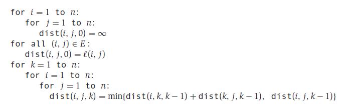
A better solution is provided by the Floyd-Warshall algorithm, which only takes O(|V|3) time using dynamic programming, by incrementally extending the intermediate vertices considered.
To calculate the product of a matrix-chain A1A2...An, n-1 matrix multiplications are needed, though different orders have different cost.
For matrix-chain A1A2A3, if the three have sizes 10-by-2, 2-by-20, and 20-by-5, respectively, then the cost of (A1A2)A3 is 10*2*20 + 10*20*5 = 1400, while the cost of A1(A2A3) is 2*20*5 + 10*2*5 = 300.
For matrix-chain Ai...Aj where each Ak has dimensions Pk-1-by-Pk, the minimum cost of the product m[i,j] corresponds to the best way to cut it into Ai...Ak and Ak+1...Aj:
    m[i, j] = 0                                                    [if i = j]
              min{ m[i,k] + m[k+1,j] + Pi-1PkPj } for i ≤ k < j     [if i < j]
Use dynamic programming to solve this problem: calculating m for sub-chains with increasing length, and using another matrix s to keep the cutting point k for each m[i,j].
Example: Given the following matrix dimensions: A1 (30-by-35), A2 (35-by-15), A3 (15-by-5), A4 (5-by-10), A5 (10-by-20), A6 (20-by-25), then the output of the program is A1A2A3A4A5A6 should be calculated as (A1(A2A3))((A4A5)A6), and the number of scalar multiplication is 15,125.
Time cost: Θ(n3), space cost: Θ(n2).
Please note that this algorithm determines the best order to carry out the matrix multiplications, without doing the multiplications themselves.
If the keys in a binary search tree have different probabilities to be searched, then a balanced tree may not give the lowest average cost (though it gives the lowest worst cost).
Using dynamic programming, binary search tree with optimal average search time can be built, in a way similar to matrix-chain multiplication.
Time cost: Θ(n3). Space cost: Θ(n2). Demo applet.