3223-03

CIS 3223. Data Structures and Algorithms

Divide-and-conquer algorithms

1. Divide-and-conquer

Solving a complex problem: divide it into subproblems, solve them, and combine the sub-solutions.

Recursion: some subproblems belong to the same type as the original problem, though with smaller problem instance size.

Recursive algorithm: (1) division, (2) recursion(s), (3) combination

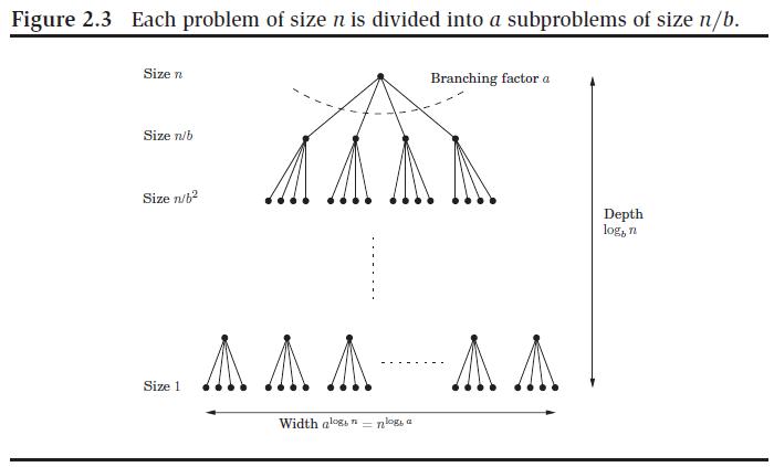
Cost: T(n) = D(n) + aT(f(n)) + C(n) = aT(f(n)) + O(G(n)), where f(n) is often n/b or n-b (b is a constant)

Boundary case: Θ(1), when n < c (a constant)

Total cost in recursion tree: Figure 2.3

With single recursion (a=1), f(n)= n-b leads to T(n) = O(nG(n)), f(n)=n/b leads to T(n) = O((log n)G(n)), though there may be tighter upper bounds.

Examples: basic arithmetic of binary numbers

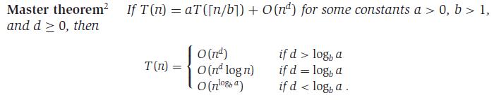
When f(n) = n/b, The Master theorem may be applicable. Special case: a=b, log_ba = 1, and the three results are O(n^d), O(n log n), and O(n), respectively.

2. Searching

Analyze the following recursive searching algorithms:

// search A[1] to A[n] for k
LINEAR-SEARCH(A, n, k)
  IF 1 > n
    THEN RETURN 0
    ELSE IF A[n] = k
           THEN RETURN n
           ELSE RETURN LINEAR-SEARCH(A, n-1, k)

If the problem instances of size n form a set {p_i}, i = 1, ..., m, and their time costs are {c_i}, then

the best cost = min(c_i), i = 1, ..., m, and the best case is the instance that has this cost
the worst cost = max(c_i), i = 1, ..., m, and the worst case is the instance that has this cost
the average cost = ΣPr(p_i)c_i, i = 1, ..., m, and especially, when all instances have the same probability, (Σc_i)/m

// search A[p] to A[r] for k when A is sorted
BINARY-SEARCH(A, p, r, k)
  IF p > r
    THEN RETURN 0
    ELSE q <- (p + r) / 2
         IF A[q] = k
           THEN RETURN q
           ELSE IF A[q] > k
                  THEN RETURN BINARY-SEARCH(A, p, q-1, k)
                  ELSE RETURN BINARY-SEARCH(A, q+1, r, k)

3. Sorting

Analyze the following recursive sorting algorithms:

// sort A[1] to A[n]
INSERTION-SORT(A, n)
  IF n > 1
    THEN INSERTION-SORT(A, n-1)
         INSERTION(A, n)

// sort A[1] to A[n]
SELECTION-SORT(A, n)
  IF n > 1
    THEN SELECTION(A, n)
         SELECTION-SORT(A, n-1)

// sort A[p] to A[r]
MERGE-SORT(A, p, r)
  IF p < r
    THEN q <- (p + r) / 2
         MERGE-SORT(A, p, q)
         MERGE-SORT(A, q+1, r)
         MERGE(A, p, q, r)

// sort A[p] to A[r]
QUICK-SORT(A, p, r)
  IF p < r
    THEN q <- PARTITION(A, p, r)
         QUICK-SORT(A, p, q-1)
         QUICK-SORT(A, q+1, r)

4. Partition and Median

The selection problem: given n numbers, find

the smallest number
the largest number
both the smallest and the largest
both the smallest and the second smallest
the ith smallest number
the (n/c)th smallest number (if c=2, it is the median)

Selection by sorting: O(n log n)

Selection by partition

Pivot value choice: middle values leads to T(n) = T(n/2) + O(n) = O(n), boundary values lead to T(n) = T(n-1) + O(n) = O(n²)

A randomly chosen pivot has 50% chance of being within the 25th to the 75th percentile, which is considered as a good pivot. In average, every two partitions reduces T(n) to T(3n/4), so the expected cost is T(n) ≤ T(3n/4) + O(n) = O(n). Note: T(n) = T(n/b) + O(n) = O(n) for all b > 1.

Similarly, using random pivot in QUICK-SORT leads to an average cost of O(n log n).

Once again: best case, worst case, and average case.