We have seen an example of bypassing the concurrency/reliability problem in a limited context: Atomic Transactions. As you remember, we can access a distributed data base using transactions without having to worry about concurrency (locks applied automatically) or about crashes (system maintains logs and uses commit protocols). Here we will discuss another example of bypassing the concurrency+ reliability problem in another limited context for truly massive data and work load.
We all know how Google search operates. It proceeds as follows
The interesting thing is that what started as a search specific approach has resulted in systems and a programming model that is proving extremely valuable in solving more general problems involving massive data sets and complex computations.
We will later look at the Google Page Ranking algorithm as an example of large computation that is run in the Google infrastructure using the Map Reduce programming model].
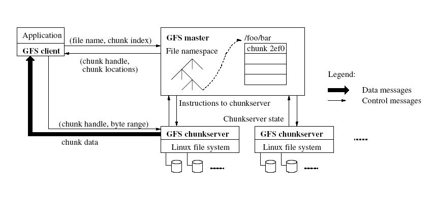
There is a single master and many chunkservers. Since the master is a single point of failure we will need to examine later the ways in which it is made fault tolerant. It maintains permanent metadata about the files:
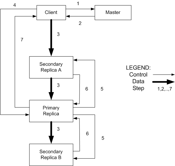
Let's examine how a client reads from a file at a specified cursor position.
Let's now look at the more complex write operation:
Let's now consider append. It proceeds as in the first 3 steps of the write operation. Then when it sends the request to the primary, the primary checks if the appended data fits in the current chunk. If not, it fills the current chunk with filler data and asks the replicas to do the same. Then it tells the client to try the operation again on the next chunk. Otherwise it appends the data to its replica and asks the secondaries to do the same at the same exact offset. Then when all secondaries acknowledge success it reports success to the client. Otherwise it reports failure and the client is supposed to retry the operation. In other words, the file may contain filler gaps, partial writes, even multiple copies of same data (caused by retry). It is a kind of at-least-once semantics.
It is important to note that the consistency of GFS does not coincide with intuitive notion of consistency [the result of a read reflects a sequential time ordered execution of the mutations that have preceded the read]. But it is adeguate to fullfil use goals for clients that have been written with logic to go around the pittfalls. Successfull mutations taking place sequentially will result in the same correct data being available at all replicas. But concurrent successful mutations caused by different clients may result in the same data in all replicas, but not the same as the data corresponding to a possible sequential execution of these mutations (i.e. some chunk may contain partial data of multiple concurrent mutations).
There are many more complexities in the Google File System. I will not deal with them. I will only mention that some locking facilities are provided and then go back to the problem of a single master for the system. To go around the possibility of failures the master uses a persistent operation log where it will record all changes in the metadata. This log, for reliability, is replicated. No change will be visible to a client unless it has first been recorded in the log and its replica(s). The master in case of crashes will be able to recover by replaying the log. And to speed up recovery the master state will be regularly checkpointed to allow for quicker recovery. It will also need to re-build its cache with handle to location map by querying the chunk servers.
Map and reduce are pure functions. Map given as argument a key, value pair produces a set of key, value pairs. The type of the map input key (the input key type) and of the map output keys (intermediate key type) may be the same or different. The same for the values (input value type and intermediate value type). The reduce function takes as argument a pair consisting of an intermediate key and a list of of intermediate values and produces a value (output value type - this type may itself be a key, value pair). All the keys and values are represented as strings.
To have an immediate feeling of what map and reduce may be here is the "Hello World" program for MapReduce: WordCount
	map(String name, String document):
	 // key: document name
	 // value: document contents
	 for each word w in document:
	   EmitIntermediate(w, "1");

	reduce(String word, Iterator partialCounts):
	 // key: a word
	 // values: a list of aggregated partial counts
	 //	here seen as an iterator on the list
	 int result = 0;
	 for each v in partialCounts:
	   result += ParseInt(v);
	 Emit(AsString(result));
As you see, the input pair has form [URL of a document, document content], the intermediate pairs produced by map have form [word, 1]. To reduce are given pairs of the form [word, (1, 1, ..., 1)] where the 1s are obtained from all the pairs generated by a map function that have that word as first component. It then produces the value [word, count], where count is the sum of the 1s. In other words, we give to map an URL and the corresponding document, and map from it produces pairs consisting of the words in the document and 1. Then in an intermediate stage all the pairs with the same word are put together to produce the pair [word, (1,1,..,1)] which is given to reduce which from it produces the pair [word, sum-of-the-ones].
A MapReduce program will be set up by chosing the number M of Map tasks (usually in the thousands) and the
number R of reduce tasks (usually in the hundreds). [By the way, each map task is implemented
as a real task, and the same for reduce tasks.]. An input reader possibly written by the user will
partition the input data into M splits and feed them to the M map tasks. The map task will
produce the intermediate pairs and place them into buffer storage. Then a partition program, usually
selected by the user for example to hash the intermediate keys into R values, will place in local disk
the resulting R partitions and will inform the R reduce tasks as to the location
of the partitions (in reality it informs the master task that will in turn inform the reduce tasks).
The reduce tasks will read the intermediate pairs that have been assigned to them,
sort them using the compare function specified by the user and collect into a list
the values associated with each intermediate key, then it will
apply the reduce function to the resulting pairs.
The result will usually be given to an output writer for writing to
global stable storage as R files.
A MapReduce computation can be described by the following diagrams which emphasize different aspects of
the computation.
This diagram expresses the computation flow we described above, from input data in global persistent storage, thru computation with an intermediate stage with persistent storage, to output data in global storage.
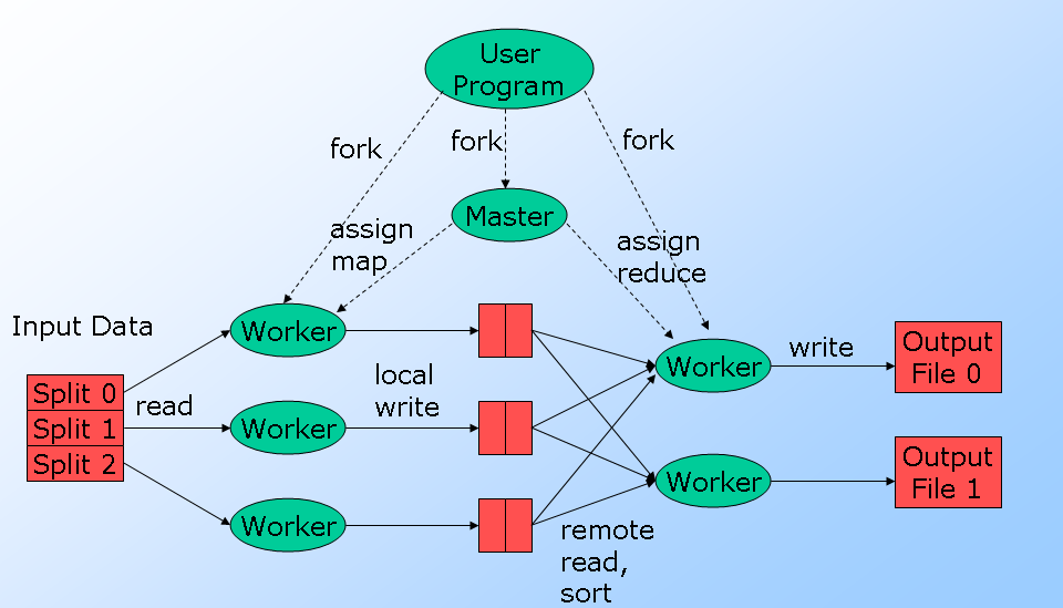
This diagram emphasizes the tasks being executed.
The user program results into worker tasks (M map tasks and R reduce tasks) plus a
master task coordinating and supervising the work of the worker tasks. The system schedules
the worker tasks on the nodes of the cluster trying to optimize placement to minimize communication overhead.
The master communicates with the workers using a heartbeat protocol.
The reduce tasks cannot start the reduce activity until the map tasks are completed.
If a map or reduce tasks crashes, the master will start a new copy of that task. If a map
task is particularly slow the master may start another map task to do the same computation.
For a given input split the reduce tasks will accept the output of the first completed map
task assigned to that split.
The master may even decide, in the case that some split results in multiple crashes,
to complete the computation without including that split in the computation.
The essential message of this diagram is that the MapReduce programmer need not worry about
issues of concurrency and fault-tolerance since all scheduling and monitoring and reexecution of worker
tasks is managed by the MapReduce master. The master is as usual a single point
of failure so its execution must be supported by a replicated log that will allow us to recover the
computation in case that the master crashes.
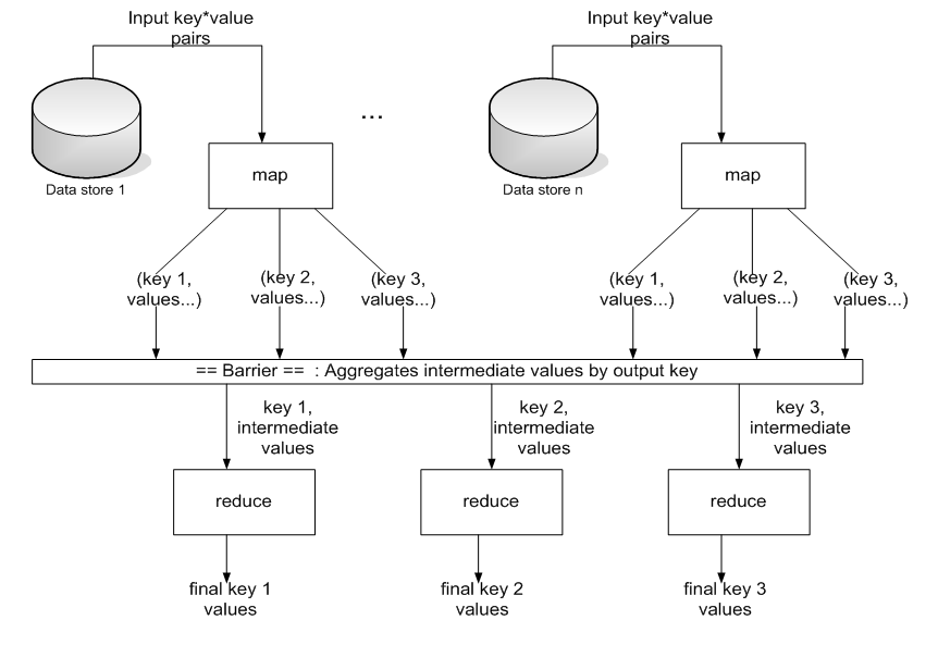
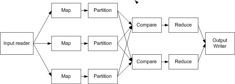
This third diagram makes a bit clearer how the reduce tasks, if they receive an intermediate key X then they receive all pairs that have intermediate key X.
A computation may involve, as in the case of WordCount, a single pass Map-Reduce.
But many computations require multiple passes each executed as a Map-Reduce computations.
The PageRank computation used by the Google Search is an example of a multi pass map-reduce computation.
We will examine it next
![]()
We can define T[h,k] as the ratio between the number of arcs going from h to k divided by the total number of arcs leaving h. So for example we will have T[1,3] = 0.4. The problem with this choice is node 4 which has no successors and that would give us a row of T filled with zeros. To go around this problem we assume that from 4 we may go with equal probability to any of the nodes, i.e with probability 1/6. The transition matrix for the given graph becomes
| 0 | 1 | 0 | 0 | 0 | 0 |
| 0 | 0 | 0.2 | 0.4 | 0.2 | 0.2 |
| 0.5 | 0 | 0 | 0 | 0.5 | 0 |
| 0.5 | 0 | 0 | 0 | 0 | 0.5 |
| 0.166 | 0.166 | 0.166 | 0.166 | 0.166 | 0.166 |
| 0 | 0 | 1 | 0 | 0 | 0 |
T'[h, k] = (1-d)/N + d * T[h, k]where d is usually chosen to be 0.85. For simplicity this new transition probability is again called T and in our example is
| 0.025 | 0.875 | 0.025 | 0.025 | 0.025 | 0.025 |
| 0.025 | 0.025 | 0.195 | 0.365 | 0.195 | 0.195 |
| 0.450 | 0.025 | 0.025 | 0.025 | 0.450 | 0.025 |
| 0.450 | 0.025 | 0.025 | 0.025 | 0.025 | 0.450 |
| 0.166 | 0.166 | 0.166 | 0.166 | 0.166 | 0.166 |
| 0.025 | 0.025 | 0.875 | 0.025 | 0.025 | 0.025 |
We can use this transition matrix to determine the probability, starting at node h (for simplicity let's
assume that h is 0) to end at node k in one
step, by multiplying the matrix T by the row vector [1,0,0,0,0,0] obtaining
the row vector [0.025,0.875,0.025,0.025,0.025,0.025]. In turn the probability of being at page k after 2
steps will be
obtained by multiplying T by this last row vector and so on.
It can be proven that the iteration converges to a result that is independent of our initial choice for h
(we had chosen h = 0).
All this is nice and good for small graphs, but what to do when the graph has hundreds of
millions of vertices? Brin and Page suggested an alternative iterative procedure to compute the page rank.
They used the following formula
	PR(T) = (1-d) + d * SUM(PR(Th)/C(Th))
where
	PR is the page rank of the page under consideration, T
	d is a tunable parameter corresponding to the idea that user do not just follow links,
		they also jump to a new page "randomly". Usually d is taken to be 0.85
	Th is a page with a link to T
	C(Th) is the number of out links from Th
then the iterative procedure starts with an initial assumption on the value of PR and determines a new distribution using the above formula, that is
PRk+1(T) = (1-d) + d * SUM(PRk(Th)/C(Th))Usually are made 20 or 30 iterations.
Now at last we get back to the PageRank computation using MapReduce. The computation is done in two phases.
PHASE 1:
	It consists of a single MapReduce computation

	The input consists of (URL, page content) pairs
	Map takes as input a (URL, page content) pair and produces the pair
		(URL, (PRinitial, list-of-all urls pointed to from URL))
	Reduce is the identity function

PHASE 2:
	It carries out MapReduce iterations until a convergence criterion has been reached.
	The kth iteration has the following form

	The input in the first iteration consists of pairs as were produced by Phase 1,
	in successive iterations it consists of the output of the previous iteration.

	Map takes as input a pair (URL, (PRk(URL), url-list of all the urls pointed to from URL))
		and produces the pair
			(URL, url-list)
		and, for each url u in url-list, the pair
			(u, PRk(URL)/Cardinality_of_url-list)
	Reduce for a given url u will sum up all values of the second kind of pair, multiply
		the sum by d and add 1-d to it obtaining a value which of course is
		PRk+1(u)
		It will then output the pair
			(u, (PRk+1(u), url-list)) // this url-list is obtained from the (URL, url-list) pairs
						// where URL is now u
As you see, it is not a trivial program, but it is feasible because the many map tasks can be done in parallel and the same is true for the reduce tasks.
The row is the fundamental entity of Bigtable. Operations on a row are atomic, even better, groups of operations can be applied atomically to a row. Here are two examples of use of a Bigtable written in C++:
Writing to Bigtable:

	// Open the table
	Table *T = OpenOrDie("bigtable/web/webtable");

	// Write a new anchor and delete an old anchor
	RowMutation r1(T, "com.cnn.www");
	r1.Set("anchor:www.c-span.org", "CNN");
	r1.Delete("anchor:www.abc.com");
	Operation op;
	Apply(&op, &r1);

Reading from Bigtable:

	Scanner scanner(T);
	ScanStream *stream;
	stream = scanner.FetchColumnFamily("anchor");
	stream->setReturnAllVersios();
	scanner.Lookup("comm.cnn.www");
	for ( ; !stream->Done(); stream->Next()) {
		printf("%s %s %11d %s\n",
			scanner->RowName(),
			stream->ColumnName(),
			stream->MicroTimestamp(),
			stream->Value());
	}
A client may request Bigtable to execute scripts within the Bigtable system itself, i.e. close to the data.
These scripts are written in a language called Sawzall
which can read but not modify the Bigtable store.
A table is split into tablets where each tablet is a contiguous set of rows.
Tablets are the unit of distribution, they play the same role in Bigtable as chunks in GFS.
As in GFS we had a master and chunkservers, in Bigtable we have a master and
tabletservers. Usually a tablet is
~200MB and a tabletserver holds a few hundred tablets. If a tabletserver crashes, its tablets are distributed
equally to the remaining tabletservers. A table may consist of hundreds of thousands of tablets.
A basic problem is to map a row key of a table to the tablet that contains the specified row.
The indexing structure required for this is not a centralized data structure, it is instead treated as a METADATA
table decomposed itself into tablets that form a 3-level hierarchical structure.
Bigtable makes use of the Chubby distributed lock service:
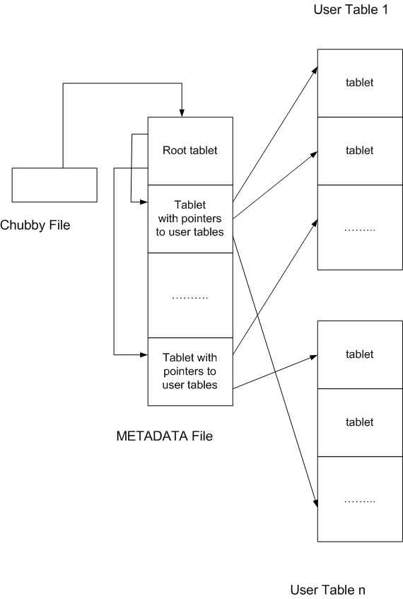
Keys in the index structure encode the pair (table identifier, index of the last row of the tablet) and the corresponding value is the pair ip-address X port of the correct tabletserver. Once at the correct tabletserver one has a second local map from row-id X column-family X column-qualifier X time-stamp to the appropriate cell content. If the time-stamp is absent then it is intended the most recent value.
The Bigtable master, like the master in GFS, is not involved in data transfer operations. Instead it is responsible to
The master does not maintain a persistent indexing structure specifying the assignment of tablets to tabletservers. Instead the master initially determines as follows the assignment of tablets to tabletservers
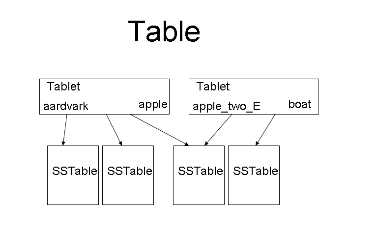
We have seen that a table is partitioned into tablets. In turn a tablet is decomposed into SSTables which are stored within GFS. Tablets may share some SSTables. The following drawing shows this hierarchy.
In turn an SSTable has an internal structure as you can see here.
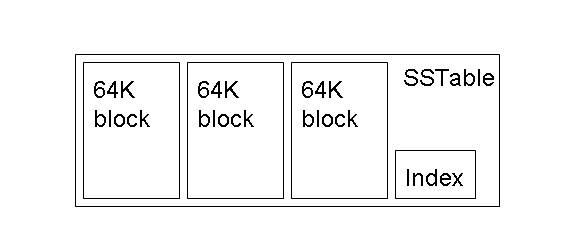
The data in an SSTable consists of pairs (key, value) and is immutable (i.e. once an SSTable is created, it is not modified, if necessary a new version will be created). The index uses the keys that you met before: row-id X column-family X column-qualifier X time-stamp. The processing of tablets and SSTables is complex and beyond what we want to discuss, but an introduction is provided by this diagram and the discussion following it.
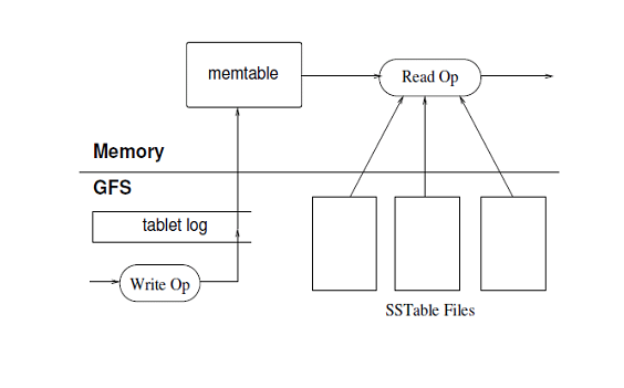
Bigtable keeps in a core data structure, memtable, much of the information needed to use a tablet. Read operations will be done reading from memtable and, for what not there, from blocks within GFS. Write operations will be recorded in a tablet log kept within GFS and then it will update the memtable. From time to time (the memtable gets too large) the tablet log and memtable are used to create a new SSTable Since a memtable may arrive to refer to a number of successive SSTables, when that number reaches a threshold the various SSTables will be merged into a compacted new SSTable.
Given distributed resources with associated values, Chubby manages their creation and naming, their deletion, their associated values, and their locking. Resources are hierarchically organized so that the service feels like a file system for small files with atomic read and write operations. Named locks allow distributed tasks to synchronize. In addition, the presence of small values associated to names allows the distributed taks to have agreed values for the important entities represented by those names.
A Chubby instance, usually called a cell consists of 5 replicas one of which acts as the master
(multiple replicas for reliability).
A cell can service thousands of clients, usually a single cluster, though it may be used in
widely distributed systems. In a cell the participants need a consensus algorithm to agree
on who will act as master and to agree on the value of inportant replicated entities. Chubby uses the
Paxos Algorithm as consensus algorithm. A majority of the participants must agree
in order to arrive to an agreement. In a cell at least 3 participants must be up for the cell to work.
When a master is selected, it remains so for a limited time (12 to 60 seconds),
it is given a lease and a new
master will not be selected until the current lease has expired. A master's lease may be extended.
A master has a fundamental role in a cell. A client accesses the Chubby server thru the DNS
service translating the name of the Chubby server to the IP address of one of the replicas.
If a client directs an operation request to a replica,
it is asked to redirect it to the master. The master informs the other participants of the write
operations it carries out
so that all participants can keep up to date their replicated copies of the shared information. Only
after a quorum of the replicas has acknowledged the write will the master acknowledge the write to the client.
Clients cache information about who is the master. If the lease of the master has expired when
a client makes a request to it, the client is informed of the identity of the new master.
If a participant crashes, after a while this is recognised by a separate Chubby component,
a new participant is selected and
started on another machine.
The DNS server is updated to reflect the new IP address.
The master becomes aware of the change by polling the DNS server and then it updates its local information.
When the new machine successfully acknowledges an operation carried out by the master it becomes available
to vote in the next election for a master.
The "files" of Chubby are available to their clients through "handles".
When a client receives a handle to a file it can subscribe to a number of events on the file, for example, when the
content of the file has been modified, or when a lock has been applied to the file. The client can specify
"call-backs" to execute when these events occur.
To speed up performance of Chubby, clients cache (for some time) the Chubby information they have previously accessed.
The Chubby cell will keep track of all the clients who have cached a particular data item and receive
KEEP-ALIVE messages from them.
If an item is modified by a client, this client will update its cache
with a write-through operation, inform the master, who will invalidate all the cached copies at the other clients.
The complexity of the Google infrastructure is very high. Supposedly by now Google has over 1 million servers and processes 20 petabytes of data each day. In our discussion we have scratched only the surface of each system. Yet we have encountered a number of general decisions and technical solutions that are worthy of emphasis.
In the future the scale of the problems that need to be solved by Google is likely to increase beyond the current cluster centered paradigm. Expect from them solutions that are more general, but are still constrained.