 CIS 307: TOPIC: Performance Evaluation
Introduction
Engineers do it. Cooks do it. But seldom programmers do it. What is it?
It is good Performance Evaluation of either an existing system or of
its design.
If an engineer estimates the need for steel in a building as a hundred
tons when two hundred are called for, he will be laughed at (or worse).
If a cook doubles the correct amount of spices in a dish, he is likely
to lose clients. But if a programmer makes estimates that are orders of
magnitude off, he feels that nothing extraordinary has happened and
many other programmers are likely to feel the same.
Yet it is not too difficult to come up with performance estimates
of times and sizes that are
fairly accurate (from 50% off to only a few % off). Thoughout this course I
do simple computations, often not more complicated than additions and
multiplications, to estimate some performance factor of a system. In your
first homework you have used a complex method of performance evaluation:
discrete-event simulation. Other methods of performance evaluation are
analytical, some involving sophisticated math like Markov models, other
are simple, as we shall now see.
Saturation and BottleNecks
We say that a server is saturated, or that it has reached
saturation when its utilization is 100% (i.e. it is busy
all the time). For example, if a disk takes 10msec to service a request,
it will saturate when it receives 100 requests per second. If a system
has many servers, we can then talk of its bottleneck, that is, of
the server that will saturate first as the load on the system increases.
Once the bottleneck saturates, also the system will saturate, i.e. it will
not be able to handle any greater load. The bottleneck of the system determines
the throughput (number of jobs completed per unit of time) of the
system. Bottleneck and system have the same bottleneck. [This discussion
assumes that we have jobs that have all the same characteristics].
Example 1: In the following system

we can execute jobs. Each job first does READ, then moves to PROCESS, then
moves to PRINT. These three phases are independent of each other in the
sense that a job can be reading while another is processing and another is
printing. Assume that a job takes 1 second to read, 4 seconds to process, and
2 seconds to print. Question: What is the (best possible) response time?
Answer: 7 seconds.
Question: What is the bottleneck in this system?
Answer: The PROCESS.
Question: How many jobs can be completed per second (at most)?
Answer: 15.
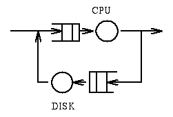
Example 2: In the following system

jobs require a total of 100msec of compute time and require 20
operations on the disk whose service time is 10msec.
Question: What is the response time? Answer: 300msec.
Question: What is the
bottleneck in this system? Answer: The disk. Question: What is the throughput
of the system? Answer: 5 jobs per second.
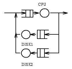
Example 3: In the following system

jobs require a total of 100msec of compute time, require 20 IO operations
on Disk 1 (whose service time is 10msec), and 50 IO operations on Disk 2
(whose service time is 5msec).
Question: What is the response time? Answer: 550msec.
Questions: What is the bottleneck? Answer:
Disk 2. Question: What is the throughput? Answer: 4 jobs per second.
Little's Law
Little's Law applies to the single server queueing system. It is the equation:
N = a * T
where:
- N is the number of jobs in the queueing system
- a is the arrival rate (the number of jobs that arrive to the system per
unit of time), and
- T is the Response or TurnAround Time for a job (total time from arrival to
departure from the system).
For example, if at the supermarket I notice that a teller has always 4
customer and that customers arrive every 2 minutes, then I know that
customers, on average will be in line for 8 minutes.
Little's Law has an intuitive foundation and it can be proven under
general assumptions as to the arrival rate of jobs, as to the service rate, and
as to the scheduling discipline. One can use it reliably.
Response Time in Round Robin Scheduling
We have seen that RR scheduling involves a quantum q. A running
process, after q seconds, is pre-empted and
placed at the end of the ready queue.
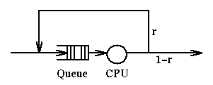
Let's assume that a process, upon completion of a quantum, has probability
r of having to run again (thus, probability 1-r of being terminated).
r is often called a Routing Probability ("route" as in which direction
to go).
How long, in total, will this program run? We can represent this system
with a picture:

If we define g(i) as the probability that a job will go i times through the
server, we have:
g(i) = (1-r)*(r**(i-1))
and the expected service time for the process, E(S), will be weighted average
of the number of quanta used at the server, say i, times the probability of
that many iterations, g(i). That is, E(S) is the sum for i from 1 to infinity
of i*q*g(i) which is:
E(S) = q/(1-r)
A more difficult question, left unanswered, is how long will it take
in this system for a job to terminate in the case that m jobs
arrive simultaneously? [May be it is m*q/(1-r)?]
Operational Analysis
We can analyze the behavior of Queueing Networks (i.e. networks of queues
and their servers) using fairly simple means. We will examine this topic by
example.
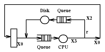
Example 1
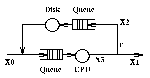
We have the
following queueing network which represents a computer system with a CPU
and a disk. When a job enters the system it goes to the CPU, whence it goes
either to disk (an IO request) or terminates. Upon completion of the IO
operation the job goes back to the CPU and things are repeated.

X0 represents the number of jobs entering the system per unit of time;
X1 represents the number of jobs exiting the system per unit of time;
X2 represents the number of jobs going to disk per unit of time;
X3 represents the number of jobs going to the CPU per unit of time.
At steady state (i.e. when the system displays the same behavior for long
periods of time) we can assume that X0=X1. By observation we determine that
in the system are present in total N jobs at a time. The service times
at the CPU and at the disk are respectively Sc and Sd.
Here are the relations that will hold in this system:
- X0+X2 = X3, because of continuity at the fork going to disk and to the exit
- X2 = r*X3, because of definition of r, X2 and X3
- N = X0*R, where R is the Response Time for this system, because
of Little's Law.
We can use these relations any way we want to compute, given the values
of some variables, the values of the remaining variables.
Example 2
Example 2 is very similar to example 1. But now the users of the systems are
all sitting at terminals. Each user request constitutes a job.

We assume:
- Each user request generates v = 20 disk requests
- Disk utilization u is 50%
- Service Time at the disk is Sd = 25ms
- There are M terminals, M = 25
- When a user receives a response, thinks for Z = 18 seconds before
submitting the next request
Question: What is the response time R? We use the equations:
- M = (R+Z)*X0, by Little's Law
- X2 = v*X0, by definition of v, X0, X2
- u = X2 / (1/Sd), by definition of u, X1, Sd
Then we get easily our response time:
- X2 = u/Sd = 0.5/0.025 = 20
- X0 = X2/v = 20/20 = 1
- R = M/X0 - Z = 25/1 - 18 = 7
Notice that it is easy to determine the maximum possible value of X2, the
saturation value, that is reached when the disk is fully utilized.
Since the service time of the disk is 25ms, the maximum value of X2 is 40
[since in a second we can have at most 40 disk operations].
As you have seen from these examples, simple performance evaluation is
very feasible, using intuition and simple math.
ingargiola.cis.temple.edu
 CIS 307: TOPIC: Performance Evaluation
 CIS 307: TOPIC: Performance Evaluation
